A thorough knowledge of the material parameters and the behavior of the material is vitally important to be able to obtain results. In order to describe the behavior of the polymers, the following properties must be examined:

The behavior of the flow of the fluids is described using the law

$$\tau = \eta \cdot \dot{\gamma} \tag{1}$$

with:

• $\tau$ = shear stress,
• $\eta$ = Viscosity and
• $\dot{\gamma}$ = shear rate.

Constant viscosities are usually found for only very small and very high shear rates for polymer melts. More often polymer melts show a pseudoplastic behavior, which can be described using the power law according to Ostwald and de Waale:

$$\tau = K \cdot \dot{\gamma}^n \tag{2}$$

In this equation:

• $K$ = Power-law coefficient and
• $n$ = Exponent of the power law (n<1).

In double logarithmic scale, the viscosity over the shear rate yields a linear profile with gradient (n-1). The gradient of this straight line is dependent on the shear rate, therefore for the value of „n“, shear rate ranges must always be given. In addition to this the shear-rate-independent zero viscosity cannot be described using the power flow law. This difficulty can be solved using the Carreau equation.

The simulation programme SIGMA offers two equations to describe the rheological behavior, firstly the Carreau–WLF (Williams, Landel-Ferry) equation and secondly the Carreau-Arrhenius equation. The equations differ in that they offer different descriptions in the temperature dependence of the viscosity [Mel98] . This difference was introduced so that data from different origins (CAMPUS; BAYMAT; VISCOSITY) is able to be entered without any conversions. The evaluation of the viscosity function with the Carreau-estimation programme offers not only the zero viscosity $a$, but the reciprocal transitional shear rate $b$, the gradient $c$, the reference temperature \( T_B \) and the standard temperature \( T_S \) which are necessary for the equation:

$$\eta = \frac{a \cdot a_T}{(1 + b \cdot a_T \cdot \dot{\gamma})^c} \tag{3}$$

In the equation:

• $a_T$ = shift factor of the temperature
• $a$ = Newton viscosity (viscosity at shear rate zero)
• $b$ = reciprocal transitional shear rate
• $c$ = gradient.

The necessary Carreau parameter viscosity at shear rate zero $a$, reciprocal transitional shear rate $b$, and gradient $c$ are determined using rheological measurements e.g. with a high pressure capillary rheometer.

The temperature shift factor $a_T$ in the equation (3) can be calculated using the Williams-Landel-Ferry (WLF) equation:

$$\lg a_T = \frac{C_1(T_B - T_S)}{C_2 + T_B - T_S} - \frac{C_1(T_1 - T_S)}{C_2 + T_1 - T_S} \tag{4}$$

In the equation:

• \( T_B \) = reference temperature
• \( T_1 \) = current Temperature
• \( T_S \) = Standard temperature, \( T_S = T_G + 50^\circ C \)
• \( C_1 = 8{,}86 \)
• \( C_2 = 101{,}6^\circ C \)

The WLF equation offers a better description than the Arrhenius-equation for amorphous polymers whose melt fluid state usually starts few degrees above the glass transition temperature. This is due to the assumption that the mobility of the polymer chains is dominated by the volume available for the movement (free volume). This free volume increases almost linearly with the difference of the current temperature to the glass transition temperature \( T_G \). If one chooses a standard temperature \( T_S \), which lies approximately \( 50^\circ C \) above the glass transition temperature \( T_G \), the parameters \( C_1 \) and \( C_2 \) in the equation (4) can be seen as being independent from the material [HKP89].

Alternatively the following equation can be used:

$$\ln a_T = \frac{C_1(T_1 - T_B)}{C_2 + T_1 - T_B} \tag{5}$$

In the equation:

• \( T_B \) = reference temperature
• \( T_1 \) = current temperature
• \( C_1 \), \( C_2 \) = adaptability constants

To be able to define the necessary Carreau parameters, measurements have to be taken, for instance, the high pressure capillary rheometer. Usually the experimental series are performed at 3 different temperatures.

In a high-pressured capillary rheometer, pre-heated material flows through a capillary with a circular cross-section. During this process, practically the total area of the interesting viscosities is measured. For low viscous fluids, long thin capillaries are used and for high viscous fluids appropriately high pressures are used. In the discontinuous method, the required pressure is applied by an external gas, gravity, or a piston. The volume flow rate is imposed, by a constant piston speed. The pressure gradient at the inlet and at the outlet is not constant due to vortex formation as a result of viscoelastic effects (Bagley-Correction), due to the change of the flow speed (Hagenbach-Correction) and due to the variation of the friction at the wall (Couette-Correction). To calculate the exact viscosity of the polymer melt, the pressure gradient is measured using two probes on a designated length in the capillary, since here, there are simple rheological flow relationships.

The calculation of both the melting behavior and the temperature development in polymer melts requires a comprehensive knowledge of the thermodynamic material behavior [HKP89]. The thermodynamic properties are dependent on both pressure and temperature and show a different material property in the solid state and in the melt state.

The following data is required for SIGMA: the crystalline melting temperature, glass transition temperature, specific heat capacity and specific enthalpy. These can be detected using the DSC (Differential Scanning Calorimetry)-analysis.

The principle is based on the measurement of the heat flow between one specimen and a comparable substance in a twin calorimeter. The sample and the reference substances are arranged symmetrically to each other so that the temperature difference is zero. Many chemical and physical transitions like melting, crystallization, oxidation or decomposition of a substance are combined with a heat flow i.e. changes in enthalpy appear. These enthalpy changes are detected by the DSC-analysis with regards to their position in the temperature range and their calorimetric magnitude. The specific heat and the enthalpy as a function of temperature can be quantified very quickly and very easily. The measurement principle is shown in the figure.

A heat flow $\dot{Q}$, drifts from the oven over a sensor (thermal resistor) to the sample pot and to the reference pot, which are usually very similar (equal in dimension and composed of the same material). The heat flow to the reference $\dot{Q}_R$ is caused due to the heat capacity of the pot material and the heat flow losses. This applies to equal pot materials, symmetry of the measuring cell and also to the specimen pot $\dot{Q}_S = \dot{Q}_R$. The sample material enclosed in the specimen pot causes an additional heat flow $\dot{H}$ (dH/ dt) that can be determined by the difference in heat flows:

$$\dot{H} = \dot{Q}_S - \dot{Q}_R = \frac{T_p - T_S}{R_t} - \frac{T_p - T_R}{R_t} = \frac{T_S - T_R}{R_t} = -\frac{\Delta T}{R_t} \tag{6}$$

Where is $\dot{H}$ = heat flow of the specimen substance $\dot{Q}_S$, resp. $\dot{Q}_R$ = heat flow to the specimen pot and reference pot, $R_t$ = thermal resistance of the sensor, $T_p$= temperature of the oven (temperature program) and $T_S$ resp. $T_R$ = reference temperature.

Partially crystalline thermoplastics do not have a fixed melting point but rather a melting range. This is due to them having different sized crystal lamellas in comparison to metals. Smaller, irregular crystallites melt at a lower temperature than larger crystallites. Characteristic for every partially crystalline polymer is the melting temperature resp. the crystallite peak temperature TK. The position of the peak on the temperature axis is identified by the start temperature ($T_A$), the peak temperature ($T_K$) and the final temperature ($T_E$) that is also important for other thermodynamic properties like specific enthalpy. For partially crystalline thermoplastics one obtains the heat flow ($T$) $\dot{H}$ over the temperature $T$ like shown in the figure:

The specific heat capacity $c$ for polymers, usually ranges from 0,1 to 5 kJ/kg*K. The figure shows clearly the specific heat capacity $c$, which is dependent on temperature for a partially crystalline polyamide.

Amorphous polymers show a different heat capacity profile $c(T)$ in contrast to partially crystalline polymers. At $T_G$ one can see an obvious change in the profile of the specific heat capacity $c$. The figure shows the specific heat capacity $c$ as a function of the temperature for amorphous polystyrene.

The material data from the DSC-analysis is used for the Simulation with SIGMA for the region above the final melting temperature $T_E$ . The approximation equation is then described by:

$$c_P(T) = c_{P0} + c_{Pm} T \tag{7}$$

Whereby the indices „0“ denotes the data on the material at a temperature of 0°C and the indices „m“ represents the slope of the material data function.

As SIGMA does not consider the influence of pressure the thermodynamic material properties should always be determined using an average pressure [Mel98].

The specific enthalpy $\Delta h$ results from the integration of the specific heat capacity $c$ within the limits $T_1$ and $T_2$ whose profile can be determined using the DSC-analysis. One now has the amount of heat required to be delivered per mass unit to the polymer.

This is:

$$\Delta h = \int_{T_1}^{T_2} c_P(T) \cdot dT \tag{8}$$

For the simulation with SIGMA one is not interested in the functional context of the specific enthalpy $\Delta h$ as a function of temperature $T$ but in the characteristic values like solid enthalpy $\Delta h_F$ and melting enthalpy $\Delta h_A$ for partially crystalline polymers or blends.

The determination of these characteristic values is shown in the figure for a partially crystalline polyamide. The melting process begins through the heat flow (melting heat) into the system and comes to an end when the final temperature $T_E$ is reached. The overall enthalpy difference $\Delta h$, that appears at this temperature ($T_E$) is the total energy required to completely melt the polymer. Through the determination of the tangent in the lower and upper temperature regions it is possible to disassemble the total enthalpy into the fractional enthalpies $\Delta h_F$ and $\Delta h_A$.

With statistical software one is able to obtain an accurate estimation in the lower temperature region through the comparison of the coefficient of determination at different temperature intervals [$T_F;T$]. The upper temperature region with the interval [$T_E;T_{max}$] is used as a calculation basis for the determination of the tangent.

Amorphous systems always show a different enthalpy profile to partially crystalline polymers as they lack melting processes. As a characteristic value for every polymer only the solid enthalpy $\Delta h_F$ is used. This is equal to the enthalpy value at the end of the melt region at the final temperature $T_E$.

Figure shows the determination of solid enthalpy the figure shows the determination of solid enthalpy $\Delta h_F$ for an amorphous polystyrene.

There is a distinct difference between steady state and non-steady state temperature fields. At steady state temperature fields the thermal conductivity $\lambda$ appears as a material parameter. The thermal conductivity is independent of temperature and for amorphous materials smaller than that of partially crystalline [Mel98].

For instance the determination of the thermal conductivity $\lambda$ can be reached with a device, namely a Thermoflixer (SWO Polymertechnik). The measuring principle is shown in Figure.

During the determination in a heated test chamber, in which the defined sample mass m is placed, the sample is in contact with a sensor. Here the sample is exposed to the heat flow $\dot{Q}$ during the time $t$.

The temperature $\delta T$ to which the sample is exposed, is recorded by the sensor. The thermal conductivity $\lambda = f(\dot{Q}, \delta T)$ can now be determined by the heat flow $\dot{Q}$ and the change in temperature $\delta T$.

The advantage of this measuring principle over the plate model (DIN 52 612) is that it offers the possibility to measure the thermal conductivity at high temperatures, which are of particular interest when using polymers. The figure shows the principle profile of the thermal conductivity $\lambda$ as a function of temperature T for partially crystalline polymers for a polypropylene.

For the simulation one needs the linear equation that describes the dotted line in the figure:

$$\lambda(T) = \lambda_0 + \lambda_m T \tag{9}$$

The values that have to be determined for eqn. 1 are the specific thermal conductivity at 0°C ($\lambda_0$) and the slope of the thermal conductivity function ($\lambda_m$).

The profile of the thermal conductivity $\lambda$ as a function of temperature for an amorphous polystyrene is shown in the figure.

In the evaluation of the DSC-analysis the profile of the input energy is drawn as a function of temperature $T$. The crystallization temperature $T_K$ for partially crystalline thermal polymers can be taken from the maximum peak of the profile curve. From the point of inflexion on the profile one can obtain the glass transitional temperature $T_G$.

If you draw the profile of the specific volume $v$ over the temperature $T$ for a partially crystalline polymer like in Figure, one recognizes that the behavior across the whole temperature range is barely if at all possible to be described mathematically.

The figure shows the profile of the specific volume v over the temperature $T$ for an amorphous polystyrene.

For the simulation of melt-dominated extruders, the temperature range above the melt temperature $T_K$, namely the glass transition temperature $T_G$, is of primary interest. For the simulation, SIGMA needs a description of the volume resp. density function in such form:

$$v(T) = v_0 + v_m T \tag{10}$$ $$\rho(T) = \rho_0 - \rho_m T \tag{11}$$

Here:

• $v_0$ = specific volume,
• $v_m$ = slope of the volume function,
• $\rho_0$ = specific density and
• $\rho_m$ = slope of the density function.

The approach to determine the bulk density $\rho_S$ (see figure) is described in DIN 53 466.

The bulk density $\rho_S$ is a value that is essentially used to determine the maximum mass throughput $\dot{m}$ of the plant and the filling degree f in the transportation of solid material. Using this one is able to determine the screw speed range needed for a desired throughput or the maximum possible throughput at a certain screw speed. The following equation is used for the evaluation:

$$\rho_s = \frac{m_1 - m_0}{V_0} \tag{12}$$

with:

• $m_1$= mass of the sample filled tank,
• $m_0$= mass of the empty tank and
• $V_0$= volume of the tank.

The solid densities can be determined according to DIN 53 479. This method (buoyancy method) compares the value of a certain sample mass of air with a fluid medium (here: distillate water $\rho_{H_2O}$=1,000 g/ cm³). The principle is shown in the figure.

In order to find the solid density of the sample one uses:

$$\rho = \frac{m_1 \cdot \rho_{H_20}}{m_1 - m_2} \tag{13}$$

with:

• $m_1$: dry mass in air
• $m_2$: sample mass in buoyant medium
• $\rho_{\mathrm{H_2O}}$: density of distilled water ($1,000,\mathrm{g/cm^3}$)

When determining the granule size, the samples are first averaged volumetrically from a total of $n$ granules and then converted into spherical form. The granule size is determined using the following equation:

$$d_{sphere} = \sqrt[3]{\frac{6 \cdot V}{\pi}} \tag{14}$$

Another option is to determine the granule diameter $d$ from a total of $n$ samples using the solid density $\rho$ and the total weight of the samples $m_{total}$. The following applies to the total of $n$ samples:

$$V_{ges} = \frac{m_{ges}}{\rho} \tag{15}$$

For one single average granule body, the equation is written as:

$$V = \frac{V_{ges}}{n} \tag{16}$$

The granule diameter $d_{sphere}$ can then be calculated by means of equation above.

Melt Volume-flow Rate

• MVR = volume/(10 min)
• Unit: [cm³/(10 min)]
• old: MVI Melt Volume Index

Melt-flow Rate

• MFR = mass/(10 min)
• Unit: [g/(10 min)]
• old: MFI Melt Flow Index

The melt index or melt flow rate is used for a quick and easy characterization of the flow behavior of polymer melts under certain pressure and temperature conditions by using a single numerical value. It indicates the amount of a melt in grams per 10 minutes. MVR / MFR according to ISO 1133 are determined by means of a capillary rheometer. While the material (granule or powder) is melted in a heated cylinder, and under a pressure caused by the bearing load, it is pressed through a defined nozzle (capillary). The values of the MVR / MFI / MFR / MVI are a measure of the viscosity of a polymer melt and allow conclusions about the degree of polymerization (average number of monomer units in a molecule). The size of nozzle, piston, cylinder and stock weights are standardized. The schematic layout of the test set is shown in the following image. The Determination of the melt mass-flow rate is analogous to the melt volume flow rate and differs in the measurement result by the melt density.

The volume or mass of the discharged polymer melt (the so-called extrudate) is determined as a function of time [MHM+05].

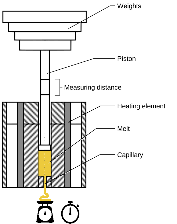
The melt flows out mass is determined by the deposition of the liquid strand at predetermined time intervals and weighing. As modified melt index the increased volume flow index MVI / MVR is strongly used indicating the extruded melt volume in 10 minutes. A major advantage of the melt volume flow rate MVR is the simple measurement of the piston travel at a known piston diameter to determine the extruded melt volume. In contrast, for the melt mass-flow rate MFR the detached molten strands have to be weighed and as result it is an additional expense for the handling. For this reason, the measurement of the mass flow rate is only used when the determination of the melt volume in case of problems during the reaction is not workable.

In order to compare MFI values among themselves, whose value must always be specified in addition to the weight used and the respective test temperature. Specifying MFI 190/2,16 for example, means that the melt index was determined at 190 ° C and a piston mass of 2,16 kg [MHM+05].

As of version SIGMA13, a model for calculating the material degradation of polypropylene has been integrated into the software. This makes it possible to visualise the molar mass degradation for the entire process as well as for the screw. The model is based on degradation tests carried out on the twin-screw extruder and the material degradation model developed at the KTP for the single-screw extruder:

$$\frac{M_n}{M_{n,0}} = \frac{1}{\exp\left(\frac{T}{T_0}\right) \cdot \left(1 + \left(\frac{Y}{Y_0}\right)^{\frac{\Pi \cdot D \cdot n}{b_0}}\right)^{\frac{t_v}{t_{v,0}}}}\tag{17}$$

The model was modified and parameterised on the basis of the findings of the experimental investigations. On the one hand, the shear rate was replaced by a shear rate averaged according to Schuler and Ansahl from the shear rates in the channel, gap and gusset:

$$\dot{\gamma}_{ia} = \frac{A_{th} \cdot 2 \cdot \pi \cdot n}{s_{ia}}\tag{18}$$

$$\dot{\gamma}_{channel} = \frac{\pi \cdot D_0 \cdot n}{H}\tag{19}$$

$$\dot{\gamma}_{rc} = \frac{\pi \cdot d_0 \cdot n}{s_R}\tag{20}$$

$$\dot{\gamma}_{res} = \omega_{ia} \cdot \dot{\gamma}_{ia} + \omega_{channel} \cdot \dot{\gamma}_{channel} + \omega_{rc} \cdot \dot{\gamma}_{rc}\tag{21}$$

$$\omega_i = \frac{A_i}{A_{free}} = \frac{A_i}{A_{ia} + A_{channel} + A_{rc}}\tag{22}$$

In addition, the residence time difference between two support points was integrated into the equation to calculate the material degradation at each support point. For the calculation of the degradation quotient from the initial molar mass and the calculated molar mass at the individual support points, the final result is:

$$\frac{M_w}{M_{w,0}} = \frac{1}{\left[ \exp\left(\frac{T}{T_0}\right) \cdot \left( 1 + \left( \frac{\dot{\gamma}_{res}}{\dot{\gamma}_0} \right)^2 \right) \right]^{\frac{\Delta t_v}{t_{v,0}}}}\tag{23}$$

Both the rheological and the thermodynamical characteristic values of a binary system (e.g. solid and melting enthalpy of polymer blends) are generally deemed as being insufficiently describable over a linear average of the data from the raw components. This means for the simulation with SIGMA that before one starts a simulation, the material data of the binary systems should be determined. This would result in numerous measurements before the simulation process actually starts. If one only has the material data for the single components, the calculations for the binary systems using SIGMA will use the material data of the single components in the following ways:

To calculate the viscosity of binary systems one can find both simple and mathematically more complex mixing rules. This is dependent on the level of accuracy required. In the simulation software SIGMA the following general mixing rules are applied. The simplest and prevalent logarithmic mixing rule is from Arrhenius:

$$\log \eta_{MIX} = w_1 \cdot \log \eta_1 + w_2 \cdot \log \eta_2 \tag{24}$$

The other one is the mixing rule according to Mantford:

$$\eta_{MIX}^{1/3.4} = w_1 \cdot \eta_1^{1/3.4} + w_2 \cdot \eta_2^{1/3.4} \tag{25}$$

The determination of the blend viscosity from the viscosity of the single components $\eta$ and the weight contents $w_i$ with SIGMA is shown in the figure.

In order to calculate the viscosity $\eta_{MIX}$ at a given shear rate $\dot{\gamma}$ for a polymer blend, the blend viscosities $\eta_{MIX 1}$ and $\eta_{MIX 2}$ have to be determined for the defined shear rates $\dot{\gamma}_1 = 0,9 \cdot \dot{\gamma}$ and $\dot{\gamma}_2 = 1,1 \cdot \dot{\gamma}$.

The approach Mantford uses is as follows:

$$\eta_{MIX 1}^{1/3.4} = w_1 \cdot \eta_{1.1}^{1/3.4} + w_2 \cdot \eta_{2.1}^{1/3.4} \tag{26}$$ $$\eta_{MIX 2}^{1/3.4} = w_1 \cdot \eta_{1.2}^{1/3.4} + w_2 \cdot \eta_{2.2}^{1/3.4} \tag{27}$$

Analogous to it the logarithm mixing rule (Arrhenius) is:

$$\log \eta_{MIX 2} = w_1 \cdot \log \eta_{1.1} + w_2 \cdot \log \eta_{2.1} \tag{28}$$ $$\log \eta_{MIX 2} = w_1 \cdot \log \eta_{1.2} + w_2 \cdot \log \eta_{2.2} \tag{29}$$

If these values are known the flow index n and the consistence K of the estimated blend segment between $\dot{\gamma}_1 = \dot{\gamma}_{MIX 1}$ and $\dot{\gamma}_2 = \dot{\gamma}_{MIX 2}$ are:

$$n = 1 + \frac{\log \left(\frac{\eta_{MIX 1}}{\eta_{MIX 2}}\right)}{\log \left(\frac{\dot{\gamma}_{MIX 1}}{\dot{\gamma}_{MIX 2}}\right)} \tag{30}$$

$$K = \frac{\eta_{MIX 1}}{\dot{\gamma}_{MIX 1}^{n-1}} \tag{31}$$

The desired viscosity $\eta_{MIX}$ results in:

$$\eta_{MIX} = K \cdot \dot{\gamma}_{MIX}^{n-1} \tag{32}$$

If the disperse Phase is available in either solid or high viscous forms one can call it a filled system. For the simulation of a filled polymer one must firstly define its basic polymer content and the size of the granules' diameter. After this the filler must be defined. Therefore data on several materials is necessary: The granule diameter d, the mass content w, the solid density $\rho$, the bulk density $\lambda_0$, the thermal conductivity of the solid $\rho_S$ and the specific heat capacity c0. As with the polymer blend the filled polymers can be defined using two different mixing equations. The former is based on the approach by Einstein:

$$\eta_{MIX} = \eta_1 \cdot (1 + 2,5 \cdot \phi_2) \tag{33}$$

and the second is based on the approach by Hashin:

$$\eta_{MIX} = \eta_1 \cdot \left[1 + 2 \cdot \frac{\phi_2}{1 - \phi_2}\right] \tag{34}$$

In these eqs. $\eta_1$ represents the viscosity of the basic polymer and $\phi_2$ refers to the volumetric content of the added component.

The experimentally crystallite melting temperatures measured for the polymer blends as well as for filled systems (compounds) are shown in the figure. For polymer blends SIGMA calculates the crystallite melt temperature $T_{K.MIX}$ from the weight contents wi and the crystalline melt temperature $T_{K i}$ as follows:

$$T_{K.MIX} = w_1 \cdot T_{K.1} + w_2 \cdot T_{K.2} \tag{35}$$

for compounds:

$$T_{K.MIX} = T_{K.1} \tag{36}$$

So the crystalline melt temperature $T_{K.MIX}$ of a filled polymer (compound) is assumed to be equal to the crystallite melt temperature $T_{K 1}$ of the basic polymer.

Figure: Crystalline melt temperature $T_{K i}$ of binary systems: polymer blends (left) and compounds (right).

In the description of the specific heat capacity c of binary systems one should use a consistent mixing rule for both the polymer blends and for the filled systems. For the specific heat capacity of the blend $c_{MIX}$ one uses:

$$c_{MIX} = w_1 \cdot c_1 + w_2 \cdot c_2 \tag{37}$$

Where the weight content $w$ and the specific heat capacity $c$ correspond to the single added component respectively.

The specific heat capacity $c_{0,MIX}$ of the blend is set to:

$$c_{0,MIX} = w_1 \cdot c_{0.1} + w_2 \cdot c_{0.2} \tag{38}$$

In the figure one can see the profile of the specific heat capacity c0 for polymer blends and filled systems.

Also the slope of the heat capacity profile $c_{m.MIX}$ for the blend is determined for both systems analogous to eqn. 37:

$$c_{m.MIX} = w_1 \cdot c_{m.1} + w_2 \cdot c_{m.2} \tag{39}$$

The relationship between the specific heat capacity cm and the weight contents for polymer blends and filled systems is shown in the figure:

Figure: Heat capacity cm of binary systems: polymer blends (left) and filled systems (right).

The specific enthalpy is set at:

$$\Delta h = w_1 \cdot \Delta h_1 + w_2 \cdot \Delta h_2 = w_1 \cdot (\Delta h_F + \Delta h_A)_1 + w_2 \cdot (\Delta h_F + \Delta h_A)_2 \tag{40}$$

Index „1“ is related to the polymer 1 and index „2“ to the polymer 2. To describe the specific enthalpy δh of filled systems (compounds) one uses the following approach:

$$\Delta h = w_1 \cdot (\Delta h_F + \Delta h_A)_1 + w_2 \cdot c_2 \cdot \Delta T \tag{41}$$

Here index „1“ is related to the polymer and index „2“ to the filler.

The solid enthalpy $\Delta h_F$ and the melt enthalpy $\Delta h_A$ for polymer blends can be determined using the enthalpy values of the basic components. For the solid enthalpy $\Delta h_{F.MIX}$ melt enthalpy of the blend $\Delta h_{A.Mix}$ one uses:

$$\Delta h_{F.MIX} = w_1 \cdot \Delta h_{F.1} + w_2 \cdot \Delta h_{F.2} \tag{42}$$

$$\Delta h_{A.MIX} = w_1 \cdot \Delta h_{A.1} + w_2 \cdot \Delta h_{A.2} \tag{43}$$

The compounds (filled system) solid enthalpy $\Delta h_{F.MIX}$ and the melt enthalpy $\Delta h_{A.MIX}$ of the blend are calculated as follows:

$$\Delta h_{F.MIX} = w_1 \cdot \Delta h_{F.1} \tag{44}$$ $$\Delta h_{A.MIX} = w_1 \cdot \Delta h_{A.1} + w_2 \cdot c_2 \cdot \Delta T \tag{45}$$

Both figures show examples for results of experimental analysis of the specific solid enthalpy $\Delta h_F$ and the specific melt enthalpy $\Delta h_A$ of binary systems.

Figure: Specific solid enthalpy $\Delta h_A$ of binary systems: polymer blends (left) and filled systems (right).

In the simulation program SIGMA the following equations are used to determine the thermal conductivity $\lambda_{MIX}$ for binary systems from the values of the single component polymers (wi,λi). For polymer blends the following equation is used:

$$\lambda_{MIX} = w_1 \cdot \lambda_1 + w_2 \cdot \lambda_2 \tag{46}$$

For filled polymers (compounds) the following relationship is assumed for the calculation of the thermal conductivity:

$$\lambda_{MIX} = \lambda_2 \cdot \frac{\lambda_1 + 2 \cdot \lambda_2 - 2 \cdot \phi_1 \cdot (\lambda_2 - \lambda_1)}{\lambda_1 + 2 \cdot \lambda_2 + \phi_1 \cdot (\lambda_2 - \lambda_1)} \tag{47}$$

The index „1“ and „2“ correspond to the mixed single components 1 and 2 when using polymer blends. When using the filled system, the index „1“ stands for the basic polymer and in the case of the added filler, the index „2“. Every component uses a linear estimation like the one mentioned in Chapter Measuring the Porosity:

$$\lambda_i = \lambda_{0i} + \lambda_{mi} \cdot T \tag{48}$$

Where λ0i is the value of the linear estimation function for the thermal conductivity of one of the components at the temperature T = 0°C and λm,i is the slope of the approximated thermal conductivity profile of the component for temperatures in the area above the melt temperature. For polymer blends the thermal conductivity of the blend λ0,MIX is:

$$\lambda_{0,MIX} = w_1 \cdot \lambda_{0,1} + w_2 \cdot \lambda_{0,2} \tag{49}$$

The slope of the thermal conductivity function λm,MIX of the blend is calculated using:

$$\lambda_{m,MIX} = w_1 \cdot \lambda_{m,1} + w_2 \cdot \lambda_{m,2} \tag{50}$$

For filled polymers (compounds) the following mixing rules result if one wants to calculate λ0,MIX and λm,MIX :

$$\lambda_{0,MIX} = \lambda_{0,2} \cdot \frac{\lambda_{0,1} + 2 \cdot \lambda_{0,2} - 2 \cdot \phi_1 \cdot (\lambda_{0,2} - \lambda_{0,1})}{\lambda_{0,1} + 2 \cdot \lambda_{0,2} + \phi_1 \cdot (\lambda_{0,2} - \lambda_{0,1})} \tag{51}$$

and

$$\lambda_{m,MIX} = \lambda_{m,2} \cdot \frac{\lambda_{m,1} + 2 \cdot \lambda_{m,2} - 2 \cdot \phi_1 \cdot (\lambda_{m,2} - \lambda_{m,1})}{\lambda_{m,1} + 2 \cdot \lambda_{m,2} + \phi_1 \cdot (\lambda_{m,2} - \lambda_{m,1})} \tag{52}$$

The solid density and the melt density ρMIX of polymer blends and compounds can be calculated by means of the densities ρi and the weight contents wi of the individual components and the following equation:

$$\frac{1}{\rho_{MIX}} = \frac{w_1}{\rho_1} + \frac{w_2}{\rho_2} \tag{53}$$

The calculation of the specific volume v of polymer blends and compounds from the specific volume vi and the weight contents wi of the single components resp. of the basic polymer and the filler are described in the following equation:

$$v_{MIX} = w_1 \cdot v_1 + w_2 \cdot v_2 \tag{54}$$

For polymer blends and filled polymers (compounds) the following mixing equations result when one wants to calculate v0MIX and vmMIX:

$$v_{0,MIX} = w_1 \cdot v_{0,1} + w_2 \cdot v_{0,2} \tag{55}$$

and

$$v_{m,MIX} = w_1 \cdot v_{m,1} + w_2 \cdot v_{m,2} \tag{56}$$

To determine the bulk density $\rho_{S.MIX}$ of binary systems like polymer blends and compounds with a granule diameter $d_1$ and $d_2$ (where $d_1 < d_2$) of the single components respective of the viscosity polymer and the filler, one must firstly make the following considerations. In the figure one can see the bulk density $\rho_{S.MIX}$ of a filler of two different particle fractions.

One must take into account that the diameter of the smaller granule particle fraction is much smaller than the granule diameter of the larger fraction (d1 « d2). If one draws the bulk density ρS MIX of a fill of two different particle fractions as a function of the weight content of the smaller fraction w1 every profile will have a maximum in the saturation concentration w1 = wSät independent of the porosity e. The degree of saturation concentration is defined as follows:

$$w_{sat} = \frac{\rho_2 \cdot (1 - \rho_{\infty}) \cdot (1 - e)}{\rho_1 + \rho_2 \cdot (1 - \rho_{\infty}) \cdot (1 - e)} \tag{57}$$

The limiting degree for a face-centred cubic sphere is:

$$p_{\infty} = \frac{V_{sphere}}{V_{total}} = \frac{\pi}{3 \cdot \sqrt{2}} \approx 0,74 \tag{58}$$

Thereby, VKugel is the volume occupied by the larger sized material (Mat 2) related to the total volume Vgesamt. The porosity e is set to e = 0,25 and is too small for the smaller material component (mat. 1) to fit in. Hence the following equation results for the saturation bulk density (bulk density of the mixing region):

$$\rho_{sat} = \rho_1 + (1 - \rho_{\infty}) \cdot (1 - e) \cdot \rho_2 \tag{59}$$

If one wants to determine the bulk density ρS MIX of binary systems using polymer blends and compounds with $d_1 < d_2$, three cases are distinguished. The strategy of the three cases is shown in the figure. The ratio of the particle fractions ($d_1/d_2$) is set to the sub division criteria for every case. Firstly one assumes two different basic approaches ($d_1 < 0,25d_2$ resp. $d_1 > 0,75d_2$) while the third basic approach is calculated by the linear average of the first two approaches in the transition zone ($0,25d_2 < d_1 < 0,75d_2$).

Bulk density of binary Systems (Polymerblends and Compounds with $d_1 < d_2$)

Case I (if $d_1 « d_2$ i. e. $d_1 < 0,25 d_2$)

• if $w < w_{Sät}$

$$\rho_{Mix} = \left(1 - \frac{w_1}{w_{Sät}}\right)\rho_1 + \frac{w_1}{w_{Sät}} \rho_{Sät}$\tag{60}$

• if $w \geq w_{Sät}$

$$\rho_{Mix} = \left(1 - \frac{1 - w_1}{1 - w_{Sät}}\right)\rho_2 + \frac{1 - w_1}{1 - w_{Sät}} \rho_{Sät}\tag{61}$$

Case II (if $d_1 > 0,75 d_2$)

$$\frac{1}{\rho_{Mix}} = \frac{w_1}{\rho_1} + \frac{w_2}{\rho_2}\tag{62}$$

Case III (if $0,25 d_2 < d_1 < 0,75 d_2$)

$$\rho_{Mix} = (\rho_{Mix I} + \rho_{Mix II}) / 2\tag{63}$$

= linear averaging of Case I and II

The interfacial tension can be determined experimentally using several methods, for example:

• „Breaking Thread“,
• „Pendant Drop“ and
• „Spinning Drop“.

The ‘breaking thread’ method is based on the theoretical description of the breakup of a liquid Newtonian thread in a Newtonian matrix. However, this method is limited to multi-component systems in which the melting temperature of the dispersed phase is higher than that of the matrix. In addition, the zero viscosity $\eta_0$ (viscosity $\eta$ at $\dot{\gamma}$ towards 0) of the matrix should not exceed 40 kPas. The following image shows the schematic structure of the test rig set up for the measurements. The heating table is flushed with nitrogen throughout the entire duration of the experiment. Before the measurement begins, the system is tempered in the heating table for approximately 10 minutes at 220 °C to minimise retardation effects during melting. The system is then heated to the desired test temperature. As soon as the filament has melted, capillary waves form at its interface with the matrix. The entire process is recorded with a CCD camera.

This sinus shaped capillary wave or thread constriction is analyzed and entered into a computer in intervals.

From the thread the initial diameter $D_0$, the wavelength $\lambda$ the largest and the smallest thread diameter $D_{max}$ and $D_{min}$ are measured. The figure shows the principle shape of such capillary waves with their characterizing values.

Figure: Scematic of a capillary wave with its characterizing values

The interfacial tension $\gamma_{12}$ is a function of the amplitude growth rate $q$, the dimensionless growth rate $Ω$, the matrix viscosity $\eta_c$ and the outer thread diameter $D_0$ . This is written as follows:

$$\gamma_{12} = \frac{q \cdot \eta_c \cdot D_0}{\Omega(p,X)} \tag{64}$$

The amplitude growth rate $q$ can be determined by the slope $S$ of the relative amplitude $\log \left(2 \cdot \frac{a_s}{D_0}\right)$ over the time (see figure):

$$q = S \cdot \ln 10 \tag{65}$$

Figure: Profile of the relative amplitude over the time for a PPT/B4 –and a PPH/B3 -blend at 260 °C

The following equation is used to obtain a value for the vibration amplitude:

$$a_s = \frac{D_{max} - D_{min}}{4} \tag{66}$$

To calculate the interfacial tension $\gamma_{12}$ , the dimensionless growth rate $\Omega(p,X)$ is used. The following rules are applied for the viscosity ratio:

$$p = \frac{\eta_d}{\eta_c} \tag{67}$$

And for the wave number, which is measured using:

$$X = \frac{\pi \cdot D_0}{\lambda} \tag{68}$$

The figure shows the profile of the dimensionless growth rate $Ω$ independent from viscosity $p$ and the wave number $X$. The solid line represents the maximum value of the dimensionless growth rate $Ω_m$.

If one plots the determined $\gamma_{12}$-values for the different temperatures $T$, the pair of values above the crystalline melt temperature $T_K$ for partially crystalline polymer pairs, the glass transition temperature $T_G$ for amorphous polymer pairs, are approximated through a linear approximation function in the following way:

$$\gamma_{12}(T) = \gamma_{12,0} - \gamma_{12,m} \cdot T \tag{69}$$

The value γ12,0 is the point of intersection of the approximation function with the co-ordinate axis while γ12,m is common with the slope of this function. In the figure one can see the principle profile of the interfacial tension γ12, as a function of temperature T, for a polypropylene (PP) / polyamide (PA6)- blend.

Figure: Profile of the interfacial tension γ12 as a function of temperature T for a partially crystalline polypropylene (PP) / polyamide (PA6) – blend.

Referring to the literature one can find the approximation value $\gamma_{12,0}$ the slope of the straight line. In reality this value varies when using different polymer pairs. Only two measurements of the interfacial tension γ12, at two different temperatures T are required to determine the approximation function. When using the „Breaking Thread“ method one is able to determine the interfacial tensions γ12 above the melt temperature TK with the help of the advanced approximation function with only a few experiments. The „pendant drop“ method is the most versatile and reliable process for measuring the interfacial tension of polymers. On the one hand the state of equilibrium between the polymer phases adjusts rapidly in comparison to other methods and on the other hand this method has the ability to perform the measurements in an inert atmosphere. The process is based on the optical measurement of the shape of a fluid or melt drop that is embedded with the surrounding phase in a hydrostatic equilibrium (see figure). This shape is comparable with that of a theoretically predicted shape of drop. This shape can be calculated on the basis of the Gauss-Laplace equation. The interfacial- or surface tension is then described as follows:

$$\gamma_{12} = g \cdot \Delta\rho \cdot d_1^2 \cdot \frac{1}{H} \tag{70}$$

Figure: Shape of a hanging droplet

Within equation 70 g is the gravitational acceleration, Δρ is the density difference of the polymer phases and 1/H is a correction factor whose value is dependent on the shape factor. This shape factor is determined using:

$$S = \frac{d_2}{d_1} \tag{71}$$

Therefore d1 is the largest drop diameter and d2 the drop diameter with a distance from the apex of d1. Values of the correction factor 1/H can be determined numerically using tables with the following equations:

$$\frac{1}{H} = \left(\frac{0,32720}{S^{2.56651}}\right) - 0,97553 \cdot S^2 + 0,84059 \cdot S - 0,18069 \tag{72}$$

for $0,401 \leq S \leq 0,46$,

$$\frac{1}{H} = \left(\frac{0,31968}{S^{2.39725}}\right) - 0,46898 \cdot S^2 + 0,50059 \cdot S - 0,13261 \tag{73}$$

for $0,46 \leq S \leq 0,59$,

$$\frac{1}{H} = \left(\frac{0,31522}{S^{2.62435}}\right) - 0,11714 \cdot S^2 + 0,15756 \cdot S - 0,05285 \tag{74}$$

for $0,59 \leq S \leq 0,68$,

$$\frac{1}{H} = \left(\frac{0,31345}{S^{2.61267}}\right) - 0,09155 \cdot S^2 + 0,14701 \cdot S - 0,05877 \tag{75}$$

for $0,68 \leq S \leq 0,90$ and

$$\frac{1}{H} = \left(\frac{0,30715}{S^{2.84636}}\right) - 0,69116 \cdot S^3 + 1,08315 \cdot S^2 - 0,18341 \cdot S - 0,20970 \tag{76}$$

for $0,90 \leq S \leq 1,00$.

Using these equations the interfacial or surface tension can be calculated from the values of two diameters as well as the melt densities. But it must be ensured that the melt drop is in a state of equilibrium with the surrounding phase. At low viscous Newtonian fluids this is usually the case, whereas in the case of high viscoelastic media's the process can last for hours.

Apart for the optical effort, this method is relatively simple to carry out as it does not require a great deal of apparatus. In practice however it requires a certain degree of deftness to build an analyzable drop. In addition some prerequisites and influences must be considered for the method to be a success. From equation (7) one can see that the melt densities are required to calculate the interfacial and surface tension. Though this data is barely mentioned in the literature. Therefore this data has to be determined using experiments, which can often lead to difficulties. When practicing this process one is confronted with many restrictions. When measuring the interfacial tension the melt drop is formed in the continuous melt phase of a secondary polymer. The conditions needed for an acceptable material combination are the incompatibility of the polymers as well as a not too high melt viscosity of the continuous phase that also has to be also transparent for the optical detection of the drop shape. Furthermore the formation of bubbles during the melt process due to exhausting gases or degradation phenomenon's of both phases can appear which leads to a variation in the shape of the drop and consequently to unrealistic values.

The measuring principle of the „spinning drop method“ is also based on the measurement of the shape of a drop, which is built under the influence of the centrifugal force. If a cylindrical capillary containing a drop and a specifically heavier fluid, is rotated with a constant high velocity (2000-8000 1/min) around its longitudinal axis then the drop assumes a cylindrical shape with rounded ends due to the influence of the centrifugal force (see figure)

Figure: Principle layout for measuring the interfacial tension with the spinning drop method. The drop 1 of the low weighted phase is deformed to the shape 2.

The profile of the drop is based on the interfacial, the surface tension, the difference in density and the centrifugal force. As the influence of the gravity force is negligible, the interfacial tension (surface tension) is calculated using:

$$\gamma_{12} = \frac{\Delta\rho \cdot \omega^2}{4 \cdot Q} \tag{77}$$

With the angular velocity Ω of the capillary and the constant Q:

$$L_0 = \frac{(4/3) \cdot (Q \cdot R^2 + 1)}{(Q \cdot R^3)^{1/3}} \tag{78}$$

In this equation L0 is the balance length of the rotating drop and R is the radius of the drop. This method is especially used for measuring systems with extremely low interfacial tensions. Through the development of modern engineering control technology, measures of up to 10-5 - 10-6 m*N/m have been made possible. This principle excels as the interface is not disturbed by foreign bodies. As a result a de-mixing processes can be observed. The drawback of this method is the slow justification of the equilibrium state. When a fluid with an intermediate viscosity (300-500 Pas) was measured, equilibrium was finally reached after more than 3h at 6100 1/min.

The tensile strength of agglomerates is defined as the maximum force $F_N$ related to the cross section of an agglomerate whereby the force has to operate perpendicular to the surface [Sch75]. Problems arise when calculating the tensile strength, as the agglomerates are not continuums but rather a fill of primary particles that are irregularly formed and generally arranged inordinate in the agglomerate. If one assumes that the forces in agglomerates are only transited at the contact points of the individual primary particles and the inordinate arrangement of the particles it can be said that the maximum traction of the individual primary particles $F_{Np}$ results as a function of the elongation of the agglomerates (see figure).

[Sch75]

The tensile strength results from the sum of the individual adhesive force located on the cross section of the agglomerates:

$$\sigma_z = \frac{F_{N,max}}{A} = \frac{1}{A} \sum_{i=1}^n F_{Np,i}(\Delta l) \tag{79}$$

As the behavior of the force and elongation of the agglomerates is not known in detail, this equation is not of much importance. Schubert [Sch75] identified different approaches to describe the tensile strength of agglomerates. For example the approach of Rumpf [Rum61] for statistically packed monodisperse particles:

$$\sigma_z = (1 - \varepsilon) \cdot k \cdot \frac{F_H}{A_p} = \frac{(1 - \varepsilon)}{\varepsilon} \cdot \frac{F_H}{d_p^2} \tag{80}$$

This approach excels because it does not need any adaptation factors and also has an excellent correlation with experimental results for special cases. Only the adhesive forces $F_H$ are indefinite. The formation of adhesive forces that are important is dependent on the agglomerate size, the degree of fluid saturation and the electrical potential. One can see the results comparing the adhesive forces in the calculation of the different adhesive forces of a sphere–sphere model in the figure.

[Rum74]

One recognizes that the fluid bridges and the van-der-Waals forces have the most significant influence. Electrostatic binding forces have a larger range making them important for clustering processes. Additionally one can see that the gravity influence is off balance at large particle diameters (1,6 mm). One must bear in mind that this value is calculated for a sphere. For a real system this value is much lower.

In order to measure the tensile strength, the agglomerates are positioned in the circular sample mount. After which they are compressed and twisted. After the sample mount is filled, the two halves of the device are drawn apart and the forces needed are measured. The tensile strength can be calculated by relating the force needed to rupture the sample to the cross section of the apparatus [Sch75], [Wic91], [PC97].

In the figure the tensile strength of talcum as a function of the porosity is shown as an example.

The measurements of these values were taken using a device [YFY82].

Porosity is defined using the ratio of void volume to total volume:

$$\psi = \frac{V_H}{V_{ges}} \tag{81}$$

with:

• $\psi$ = porosity,
• $V_H$ = void volume,
• $V_{ges}$ = total volume.

The porosity can differ by the look of the agglomerate without being recognized. In the figure different types of pores are shown in the model of a single particle.

There are open and closed pores, pores with a fixed diameter, pores, which continually taper, and pores, which are only accessible over narrow capillaries, as well as through flow pores. Surface roughness must be considered.

The porosity of single particles $\psi_p$ is due to pores. From a cluster of particles one gets the agglomerate porosity $\psi_a$. This is the relationship of the void volume between the particles to the agglomerate volume. The problem with this definition is the specification of the agglomerate volume with respect to the outer zones.

In the loose fill of agglomerates one can find the bulk porosity $\psi_b$, which is the relationship between the agglomerates and the total volume of the loose fill within the mold cavity. The total porosity $\psi$ is composed of individual porosities. It considers:

$$(1 - \psi) = (1 - \psi_p)(1 - \psi_a)(1 - \psi_b) \tag{82}$$

Figure: Porosity of a) single particles, b) bulk [PHS79]

From measurements one cannot not distinguish between the porosity of the primary particles $\psi_p$, the porosity of the agglomerates $\psi_a$ and the bulk porosity $\psi_b$. Densities are also usually measured. A porous material has a smaller density than the solid material $\rho_f$. The density of the individual particle $\rho_p$ is related to the porosity as follows:

$$\rho_p = (1 - \psi_p) \cdot \rho_f \tag{83}$$

The agglomerate density is:

$$\rho_a = (1 - \psi_p) \cdot (1 - \psi_a) \cdot \rho_f \tag{84}$$

Appropriately considered for the bulk density $\rho_b$:

$$\rho_b = (1 - \psi_p) \cdot (1 - \psi_a) \cdot (1 - \psi_b) \cdot \rho_f \tag{85}$$

Besides the different pore types there are also various pore sizes to be considered. In the figure, the distribution density curve of the pore radius is represented for a fill of agglomerates. Generally speaking, pore sizes can be distinguished into: single particle pores, agglomerate pores and loose material pores. In the ideal case they yield various maximums of the distribution density (multi-modal).

[PHS79]

In the determination of the porosity of the agglomerates or the individual particles, there are a range of measuring techniques at ones disposal. Mentioned here are the figure analysis and the mercury porosity techniques.

For the image analysis one or more cuts are made from an agglomerate and the ratio of the void areas to the solid material fraction are determined. With the help of sequential cuts, the difference between open and closed pores can be seen. In addition, the distribution of the values and the forming area can be determined. From a single individual sectional drawing only the value distribution for the spherical pores can be calculated. The intermediate porosity areas agree well however with the total porosity.

The method suggested by Washburn 1921 [Was21] can be used to determine the volumes of the pores and of the distribution of the pore radius. Mercury wets very badly and wraps itself around the agglomerates. The volume of the mercury, which is displaced from the agglomerate, is measured with a mercury porosity meter.

Through known solid densities, the agglomerate density yields corresponding to DIN 53193 or DIN 51057 from the displaced volume and the difference in mass. In dependence of the pressure needed, the mercury penetrates the small pores, corresponding to the Gauß-Laplace equation:

$$p = \frac{2\sigma \cos(\Theta)}{r} \tag{86}$$

with:

• $p$ = pressure,
• $\sigma$ = surface tension of the mercury,
• $\Theta$ = angle of contact of the mercury,
• $r$ = radius of pore

With this equation the distribution of the pore radius lets itself be calculated [PHS79]. At higher pressures, the compressibility of the mercury must be considered.

[Dul79] Dullien, F.A.L.: Porous Media - Fluid Transport and Pore Structure, Academic Press, 1979

[HKP89] Hensen, F.; Knappe, W.; Potente, H.: Handbuch der Kunststoff-Extrusionstechnik, Band 1, Hanser Publishers, München, Wien, 1989

[Mel98] Melisch, U.: Grundlagen zur Simulation des Förder- und Plastifizierprozesses dichtkämmender Gleichdrall-Doppelschneckenextruder; Dissertation; Universität Paderborn; 1998

[MHM+05] Menges, W.; Haberstroh, E.; Michaeli, W.; Schmachtenberg, E.: Werkstoffkunde Kunststoffe. 5., völlig überarbeitete Auflage, Carl Hanser Verlag, München Wien, 2005

[PC97] Pierrat, P.; Caram, H.S.: Tensile strength of wet granular materials, Powder Technology, 91(1997), 83-93

[PHS79] Polke, R.; Herrmann, W.; Sommer, K.: Charakterisierung von Agglomeraten, Chemie Ingenieur Technik, 51(1979)4, 283-288

[Rum61] Rumpf, H.: Agglomeration, Intern. Symposium Philadelphia, 1961, 379-418

[Rum74] Rumpf, H.: Die Wissenschaft des Agglomerierens, Chemie Ingenieur Technik, 46(1974)1, 1-11

[Sch75] Schubert, H.: Tensile Strength of Agglomerates, Powder Technology, 11(1975), 107-119

[Was21] Washburn, E.W.: Proc. Nat. Acad. Sci. U.S., 7(1921), 115

[Wic91] Wicke, R.: Agglomeratkennzeichnung und Prüfmethoden, Technische Akademie Wuppertal, Wuppertal, 1991, 1-32

[YFY82] Yokoyama, T.; Fujii, K.; Yokoyama, T.: Measurement of the tensile Strength of a Powder Bed by a Swing Method Measuring Instrument , Powder Technology, 32(1982), 44 - 52[Dul79] Dullien, F.A.L.: Porous Media - Fluid Transport and Pore Structure, Academic Press, 1979

[HKP89] Hensen, F.; Knappe, W.; Potente, H.: Handbuch der Kunststoff-Extrusionstechnik, Band 1, Hanser Publishers, München, Wien, 1989

[Mel98] Melisch, U.: Grundlagen zur Simulation des Förder- und Plastifizierprozesses dichtkämmender Gleichdrall-Doppelschneckenextruder; Dissertation; Universität Paderborn; 1998

[MHM+05] Menges, W.; Haberstroh, E.; Michaeli, W.; Schmachtenberg, E.: Werkstoffkunde Kunststoffe. 5., völlig überarbeitete Auflage, Carl Hanser Verlag, München Wien, 2005

[PC97] Pierrat, P.; Caram, H.S.: Tensile strength of wet granular materials, Powder Technology, 91(1997), 83-93

[PHS79] Polke, R.; Herrmann, W.; Sommer, K.: Charakterisierung von Agglomeraten, Chemie Ingenieur Technik, 51(1979)4, 283-288

[Rum61] Rumpf, H.: Agglomeration, Intern. Symposium Philadelphia, 1961, 379-418

[Rum74] Rumpf, H.: Die Wissenschaft des Agglomerierens, Chemie Ingenieur Technik, 46(1974)1, 1-11

[Sch75] Schubert, H.: Tensile Strength of Agglomerates, Powder Technology, 11(1975), 107-119

[Was21] Washburn, E.W.: Proc. Nat. Acad. Sci. U.S., 7(1921), 115

[Wic91] Wicke, R.: Agglomeratkennzeichnung und Prüfmethoden, Technische Akademie Wuppertal, Wuppertal, 1991, 1-32

[YFY82] Yokoyama, T.; Fujii, K.; Yokoyama, T.: Measurement of the tensile Strength of a Powder Bed by a Swing Method Measuring Instrument , Powder Technology, 32(1982), 44 - 52