Inhaltsverzeichnis
SIGMA3D-Interface
This section is divided into:
- Pre Processing (configuration of geometry, process parameters, solver settings)
- Solving (starting and monitoring the Extrud3D solver)
- Post Processing (slices, rendered geometry, particle tracking, report generation, result review)
Pre-Processing
Before a simulation can be started, a SIGMA3D configuration has to be created and parameterized.
Opening the SIGMA3D configuration
Command path: Simulation > open SIGMA3D-configuration
When the command is executed, a dialog appears in which the configuration can be assigned to an existing process or created without process assignment.
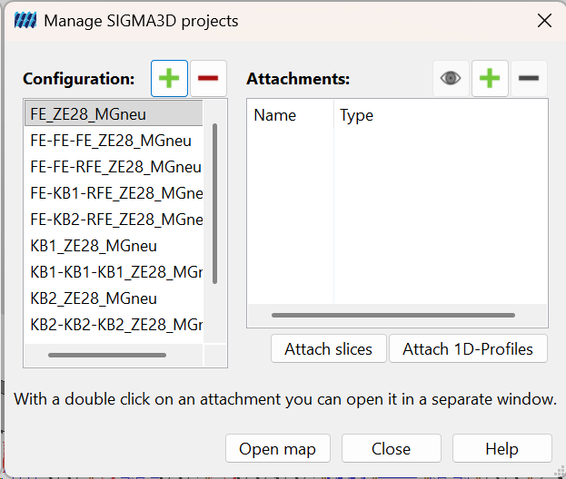
In the Manage SIGMA3D projects dialog, the following functions are available (see screenshot):
- Select an existing configuration in the Configuration list.
- Manage entries using Add (+) and Remove (-).
- Manage result attachments in the Attachments area.
- Attach generated result objects via:
- Attach slices
- Attach 1D-Profiles
- Open the result folder via Open map.
- Double-click an attachment to open it in a separate window.
After selecting or creating a configuration, the SIGMA3D configuration dialog opens.
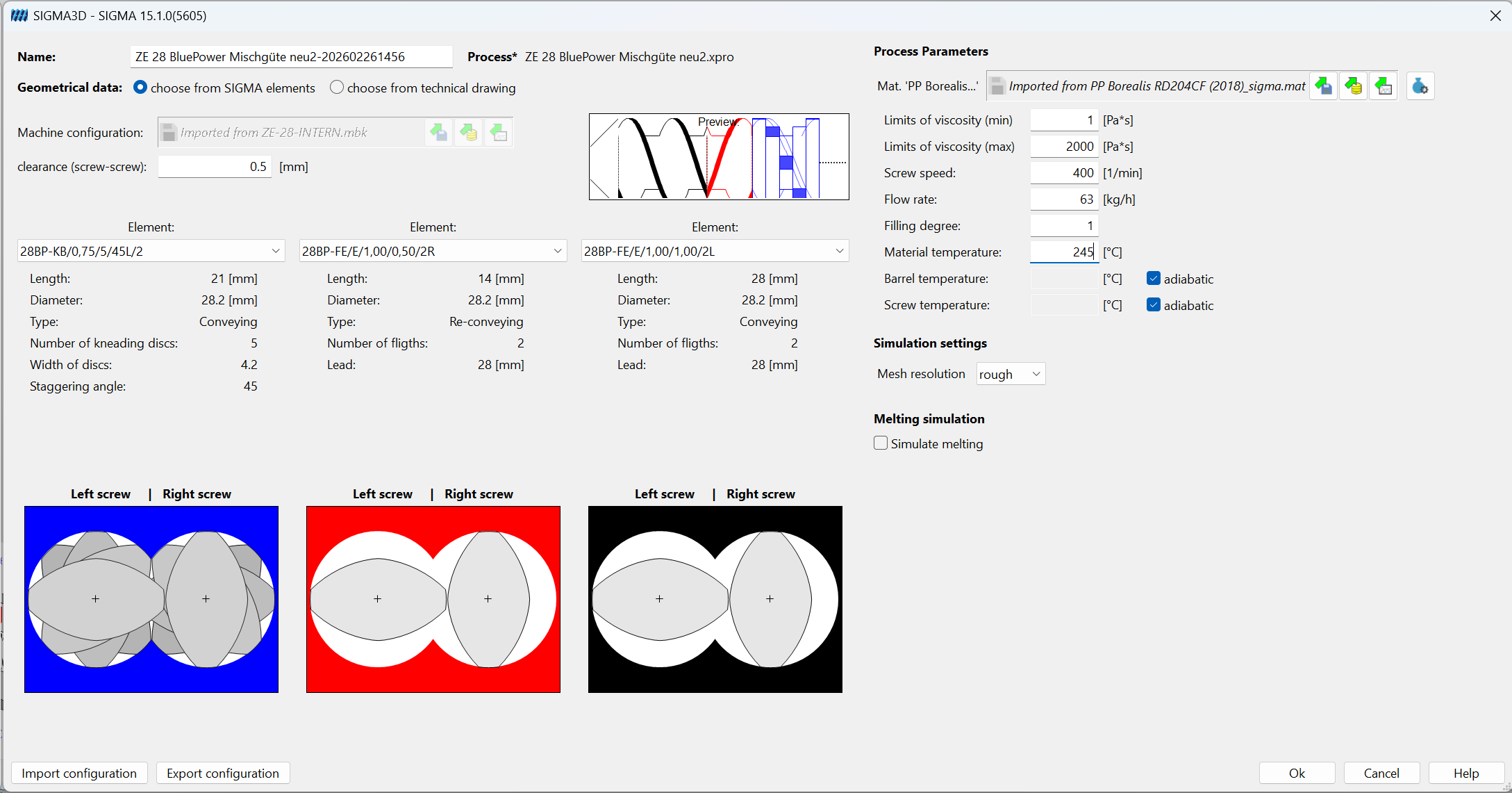
Configuration dialog overview
The configuration dialog contains all settings required to define the numerical simulation. If the configuration is assigned to a SIGMA process, machine and process data may already be pre-filled.
General data
At the top of the dialog the following information is shown:
- Name of the SIGMA3D configuration
- Assigned Process
Geometrical data source
Under Geometrical data, two options are available:
- choose from SIGMA elements : Use standard SIGMA screw elements machine construction kit.
- choose from technical drawing : Use imported CAD geometry (OBJ file).
When choose from SIGMA elements is selected:
- A Machine configuration can be loaded.
- The clearance (screw-screw) must be defined (unit: mm).
- Up to three element pairs can be selected for the simulation domain.
- For each selected element, the dialog displays geometric properties such as:
- Length
- Diameter
- Type (e.g. conveying, re-conveying)
- Number of flights / kneading discs
- Lead / width of discs / staggering angle (depending on element type)
The lower part of the window shows cross-sectional previews for the selected element pairs (left and right screw).
Alternatively, a CAD drawing can be used for the 3D simulation:
- Select choose from technical drawing
- Import an OBJ file
Important requirements and notes:
- The imported file must contain one screw only
- Additional reconstruction parameters are required to restore the real machine dimensions
- Ensure that the geometry orientation and dimensions are consistent with the machine coordinate system used in SIGMA3D
Process Parameters
The Process Parameters panel (right side of the dialog) contains the physical and operating conditions for the simulation. Typical fields include:
- Material (imported SIGMA material data)
- Limits of viscosity (min / max) [Pa·s]
- Screw speed [1/min]
- Flow rate [kg/h]
- Filling degree
- Material temperature [°C]
- Barrel temperature [°C]
- Screw temperature [°C]
For barrel and screw temperature, adiabatic checkboxes are available.
Isothermal vs. non-isothermal setup
By default, SIGMA3D is commonly configured as an isothermal simulation:
- The melt temperature is assumed constant and equal to the defined material temperature.
- Thermal energy balance is not solved in full detail.
For a non-isothermal simulation:
- Uncheck the adiabatic boxes (barrel and/or screw) as required
- Define thermal boundary conditions for barrel and screw temperatures
- Shear heating (dissipation) is taken into account
Technical consequence:
- Non-isothermal calculations are significantly more computationally intensive.
- Runtime and hardware requirements increase considerably.
Simulation settings (mesh resolution)
In the Simulation settings section, the Mesh resolution can be defined (default shown in the screenshot: rough).
SIGMA3D provides multiple mesh quality levels (five grades in total, depending on software version). Increasing mesh resolution leads to:
- finer spatial discretization
- improved local result resolution
- longer preprocessing and solver runtime
- higher CPU and RAM demand
Recommendation (engineering practice):
- Use rough/coarse meshes for initial screening and parameter studies
- Use finer meshes only for validated final evaluations or local detailed analysis
Melting simulation
Activation
Activate melting by enabling:
- Simulate melting (checkbox in section Melting simulation)
Physical model (overview)
When Melting is activated, SIGMA3D takes the solid fraction of the polymer into account and can simulate the transition from solid to melt (depending on the applied thermal boundary conditions).
If barrel and/or screw temperatures are specified (non-adiabatic conditions), the software calculates:
- heat transfer
- temperature rise
- melting progression
The melting calculation is based on the KARRENBERG melting model.
Model concept (simplified engineering description):
- The solid phase is represented as an extremely high-viscosity fluid
- Thermodynamic properties of the solid are preserved
- The transition region is modeled using a melt fraction function
- This function blends rheological and thermodynamic properties of solid and melt
- The melt fraction function is derived from the specific heat capacity vs. temperature data stored in the SIGMA material dataset
This means the melting behavior is material-specific and responds differently for different polymers.
Finalizing / saving the configuration
If the configuration is assigned to a process, the setup can be completed by clicking Ok.
A warning dialog appears:
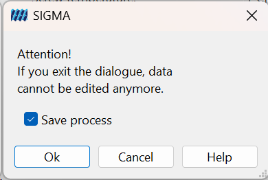
The warning indicates that after leaving the dialog, the data can no longer be edited in the same way. The option Save process is available.
Practical implication:
- Confirming with Ok saves the process and assigns the SIGMA3D configuration to the process.
- Subsequent edits may require creating or cloning a new configuration.
Import / Export configuration
At the bottom of the configuration dialog:
- Import configuration : Imports previously saved SIGMA3D configuration settings.
- Export configuration : Saves the current SIGMA3D configuration as an *.e3d file for simulation on a cluster or another workstation.
Opening the SIGMA3D process window
To start a simulation, expand the SIGMA3D tab in the project data. All created Extrud3D processes are listed there.
By double-clicking a configuration name, the SIGMA3D main window opens:
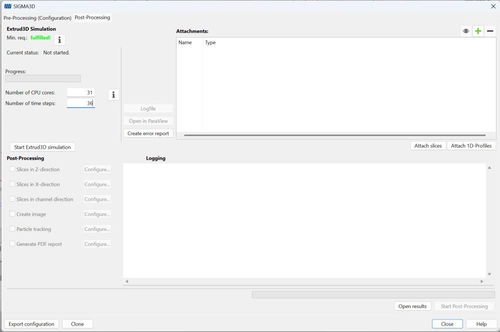
Simulation execution (Extrud3D)
The SIGMA3D main window contains two tabs:
- Pre-Processing (Configuration)
- Post-Processing
The left panel contains the Extrud3D Simulation status and controls.
Minimum requirements / status
In the Extrud3D Simulation section, the UI shows:
- Min. req. : At least a CPU with 8 cores and 32 GB RAM are necessary for a simulation
- Current status : Status of the simulation (Not started / running / crashed/ finished)
- Progress : Progress of the simulation
- Input fields for:
- Number of CPU cores
- Number of time levels
CPU cores
Set the number of CPU cores to be used for the calculation.
- The available core count depends on the workstation / server.
- At least 3 CPU cores must be available for simulation (as specified in the original workflow description).
- Higher core count generally reduces runtime, but scaling depends on problem size and hardware architecture.
Number of time steps
The field Number of time steps defines the angular discretization of one screw revolution (i.e. screw positions evaluated by the solver).
The information dialog (see screenshot) explains:
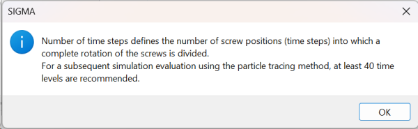
For subsequent evaluation using particle tracing, at least 36 time levels are recommended.
Starting the simulation
Start the solver by clicking: Start Extrud3D simulation
While the simulation is running, the status area updates continuously.
Example of a running simulation:
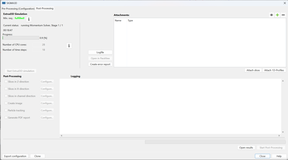
Typical runtime indicators shown in the UI:
- current solver stage
- elapsed time
- progress percentage
- active CPU core count
- configured number of time steps
Monitoring and runtime tools
During or after the simulation, the following buttons may be available (depending on status):
- Logfile Opens the solver log for diagnostics and progress review.
- Open in Para View When simulation has finished, generated results can be opened in Para View
- Create error report Creates a diagnostic package for troubleshooting.
Completed simulation
After a successful calculation, the status line changes to a stopped/completed state (wording depends on version), and the progress reaches 100.0%.
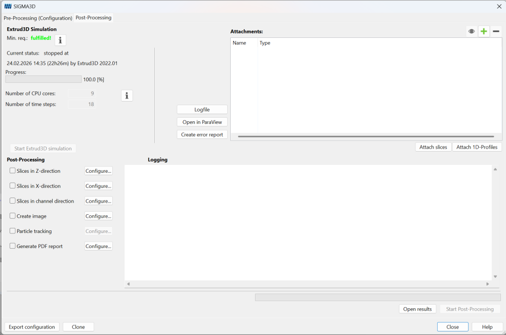
Post-Processing
After the simulation has been completed, various post-processing operations can be performed in the Post-Processing section.
The left side of the main window provides selectable post-processing tasks, each with a corresponding Configure… button.
Typical tasks shown in the UI:
- Slices in Z-direction
- Slices in X-direction
- Slices in channel direction
- Create image
- Particle tracking
- Generate PDF report
The center/right area contains:
- Attachments list (generated result objects)
- Logging window (post-processing progress/messages)
General post-processing workflow
- Select one or more post-processing tasks (checkbox)
- Open Configure… for each selected task and define parameters
- Start post-processing (button availability depends on generated outputs)
- Review generated items in Attachments
- Open results via:
- double-click attachment
- Open results
- Open in Para View (where applicable)
Slices in Z-direction
Z-slices are cross-sectional evaluations at defined axial positions.
Configuration dialog:
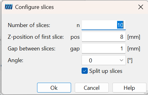
Configurable parameters (as shown in the dialog):
- Number of slices (n)
- Z-position of first slice (pos) [mm]
- Gap between slices (gap) [mm]
- Angle [°]: Screw angle position
- Split up slices (checkbox): Splits slices into cross channel and radial gap view
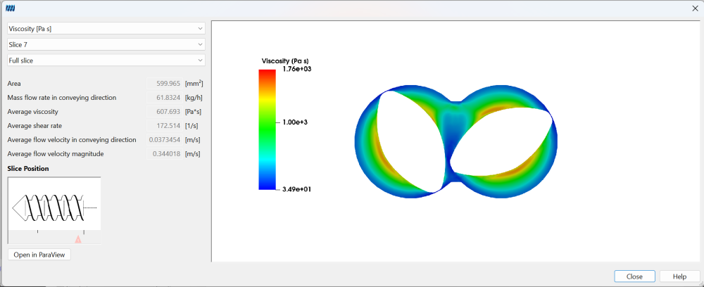
Result Slices in Z-direction
- XY / full slice contour plot with selectable variable and slice index:
Slices in X-direction
X-slices provide cross-sections normal to the X direction (depending on the internal coordinate system).
Configuration dialog:
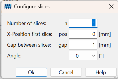
Configurable parameters:
- Number of slices (n)
- X-Position first slice (pos) [mm]
- Gap between slices (gap) [mm]
- Angle [°]: Screw angle position
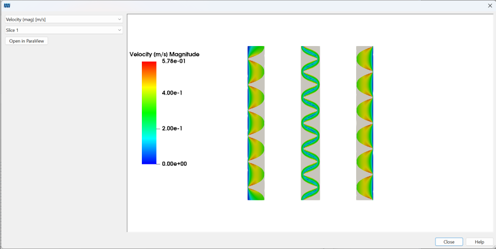
Result Slices in X-direction
X-direction slice set:
Slices in channel direction
Channel-direction slices evaluate the flow in the local screw channel coordinate system.
Configuration dialog:
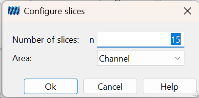
Configurable parameters:
- Number of slices (n)
- Area : Channel, cross section or both
Result view of slices in channel direction
- Single channel slice with numerical statistics:
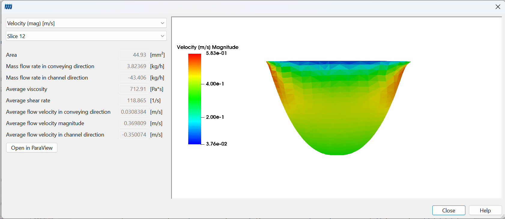
Depending on the result type, the viewer may provide:
- Variable selection (e.g. viscosity, velocity magnitude)
- Slice selection
- View mode selection (e.g. full slice)
- Numerical statistics such as:
- area
- mass flow rate (conveying direction / channel direction)
- average viscosity
- average shear rate
- average velocity components / magnitude
- Open in Para View button for advanced 3D inspection
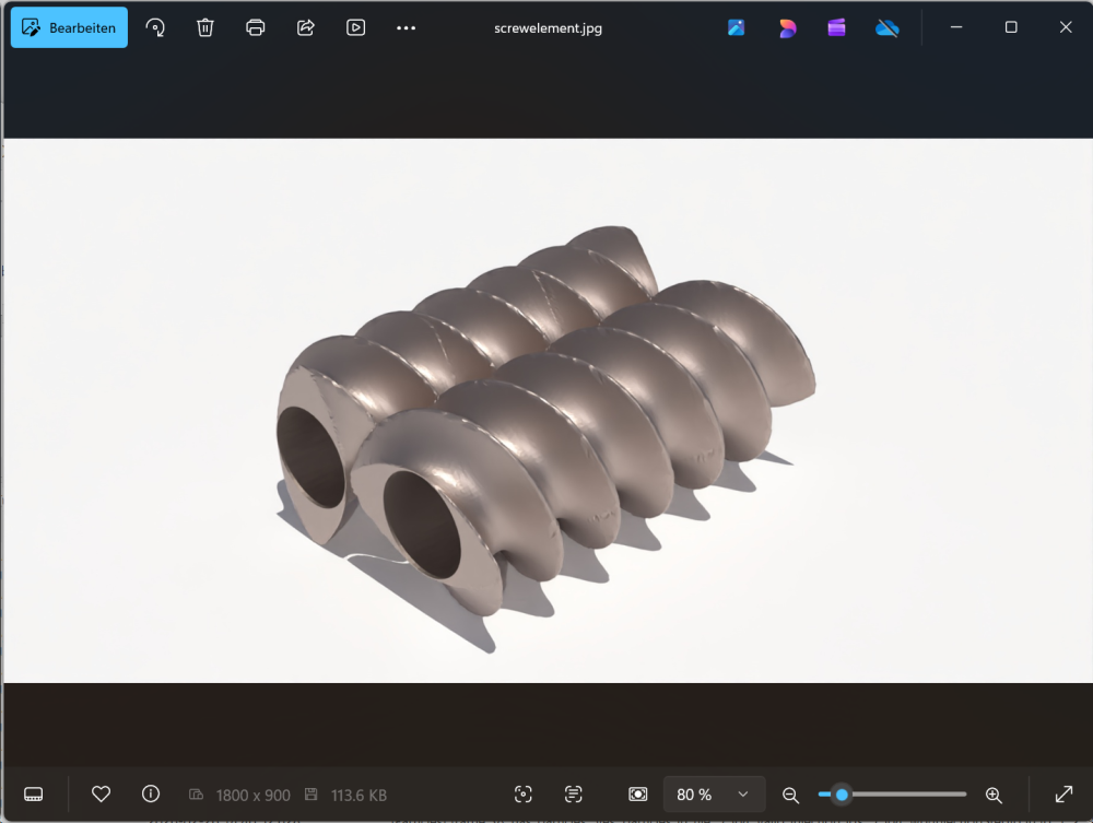
Generate rendered screw element
This function creates a rendered image of the selected screw element geometry.
Configuration dialog:
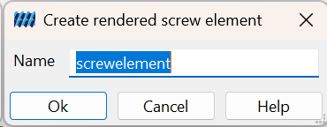
Parameter:
- Name of the generated image
Example output (rendered geometry image):
Generate PDF report
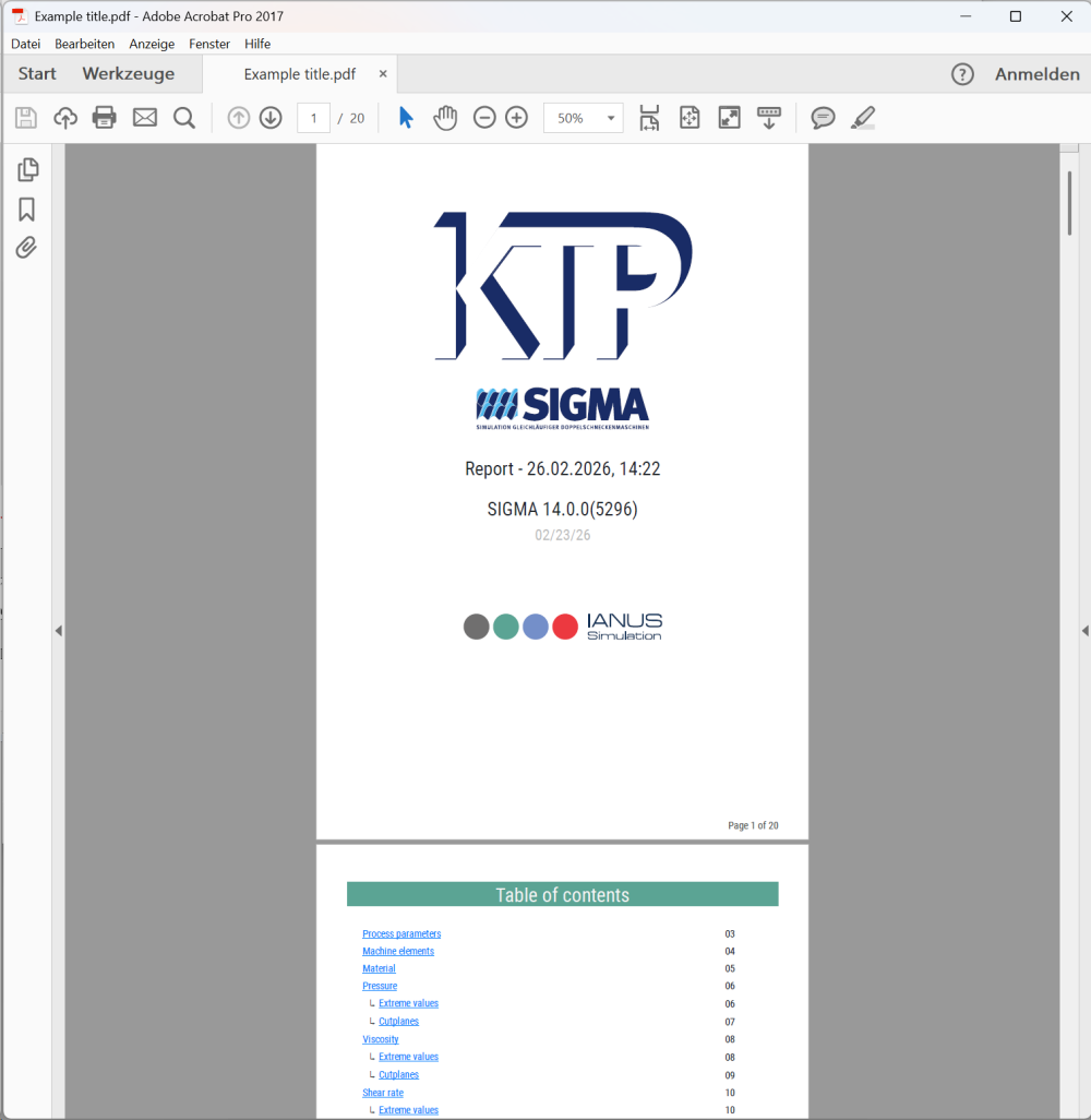
SIGMA3D can generate a PDF report with a summarized evaluation of the flow simulation.
Configuration dialog:
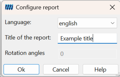
Configurable parameters:
- Language
- Title of the report
- Rotation angles (availability may depend on result setup/version)
Example output (PDF cover and table of contents):
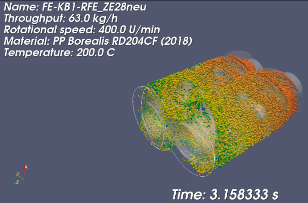
Particle tracking
Particle tracking is used to evaluate residence and transport behavior, mixing paths, and qualitative dispersive/distributive mixing effects.
Mixing ratio / Mixing quotient
The software provides a mixing quotient evaluation after running a particle tracking simulation.
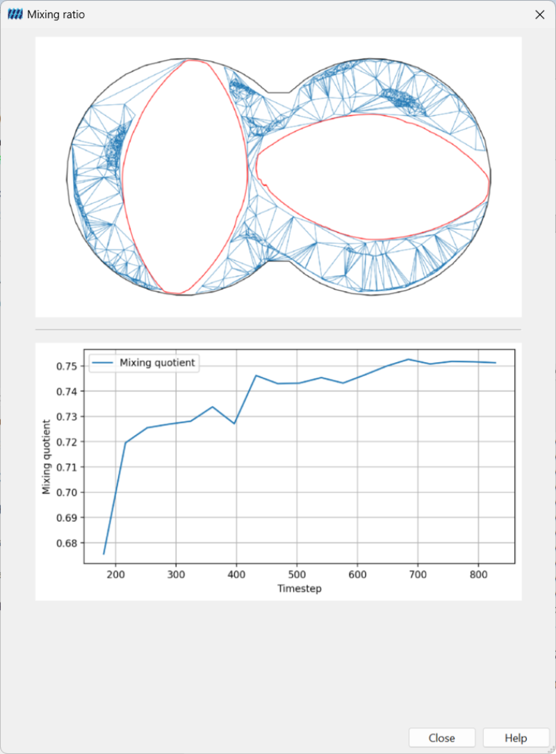
The displayed delaunay evaluation typically consists of:
- a geometric/cross-sectional representation
- a graph of mixing quotient vs. timestep
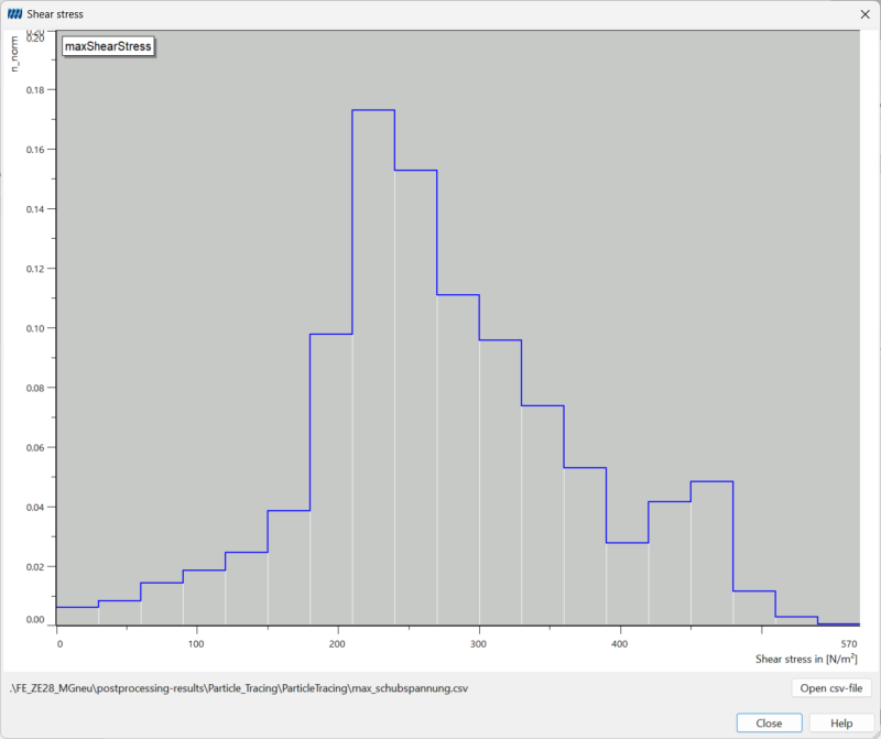
Shear stress
A shear-stress evaluation can also be generated (e.g. histogram-based output depending on the configured post-processing options and software version).
Result file location
You can access the location of generated files by:
- clicking Open results / Open map (depending on the dialog)
- using the command path:
Simulation > open SIGMA3D diagram
Managing SIGMA3D projects
To manage created SIGMA3D projects/calculations, use:
- the Manage SIGMA3D calculations icon
- or the command path:
Simulation > SIGMA3D manager
This opens the management dialog shown at the beginning of this page.
Quick access through displayed screw
As an alternative workflow, individual screw elements can be selected directly in the displayed screw configuration.
Procedure:
- Select a screw element in the visual screw layout
- Right-click the element
- Choose the option to create a SIGMA3D configuration from the context menu
This is a fast method for local element studies and comparative investigations of specific screw sections.
Recommendations for numerical simulation with SIGMA
For setup and runtime
- Start with a coarse / rough mesh for initial feasibility studies.
- Use a limited number of time steps for quick screening runs.
- Increase resolution only after the setup has been validated.
For thermal simulations
- Use non-isothermal simulation only when thermal effects are process-relevant.
- Check CPU/RAM availability before enabling thermal and melting calculations simultaneously and keep in mind, that this simulation can take time.
For particle tracking and mixing analysis
- Ensure sufficient time step resolution ( 36 for particle-tracing evaluation are recommended).