• Multi Graphic
• Create and Edit a Multi Graphic
• Diagram Views
• View of the Profiles Calculated
• The .csv-Export
• Print

**Path: **Main menu > Simulation > Multi graphic…



Multi graphics can be used to graphically compare several results (even from different processes). One can also take a closer look at individual values from the processes. Furthermore multi graphics offer the possibility to save parts of the calculation results as .csv-files to process them later with other programs (e.g. with the spread sheet Excel).

The user can use the key sequence control+’M’;. If a process window is already open the user is asked whether he wants to apply the current process. Choosing „Yes“ the multi graphic is opened with this process but more process and result files can later still be added. Otherwise a choice box is shown like with opening the multi graphic without an opened process. Here process and result files can be selected. With permanent pressing of the shift or control key more than one files can be opened at the same time.

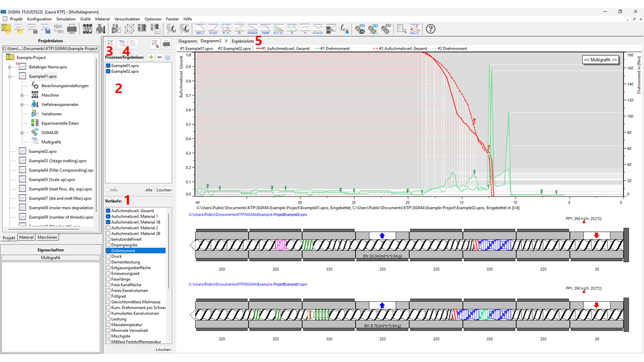
1. Selection of Curves
2. Selection of Files
3. Display Additional Diagram
4. Display Additional Event List
5. Tabs for Viewing Diagrams and Tables

Now the multi graphic window with the following areas is opened:

When pressing one of these buttons another tab with a diagram or result lists opens in the right half of the window, referred to as “page” in the following. Theoretically more than one page can be open at the same time. Afterward the user can chose from the lists which data should be shown.

All result and process files loaded in the multi graphic are listed. Through tagging or deleting tags next to the particular file name the user can choose whether the data from this source should be shown on the current page or not. It is better not to tag to many files at one time because especially diagrams are then easily confusing. The other pages are not affected by the changes.

In order to load additional results the user has to press the green -button above the list and a choice box opens. The other way round a selected file can be deleted from the list with the delete button .

Important: No files are deleted from the volume.

Here all possible profiles which appear in any source or standard profile are listed. Here again data can be added or deleted from the current view by tagging or deleting tags. If tagging is ineffective it is because fort he chosen source (results or processes) the corresponding data was not calculated. Here again not too many profiles should be shown in a graphic/table. Instead another page should be opened.

From the standard or user-defined diagrams can be chosen with the buttons below the menu bar. The “delete” button below the list deletes all tags at once.

At the right diagrams and tables are shown. With a click on the individual tab a page is brought to the front and can be configurated with the lists on the left side. Panning the tag with pressed mouse button to the edge of a window the tab is divided and more than one page can be viewed at the same time. Moving the tab on another tab moves the tab there and if needed the window splitting is annulated.

With the tabs also windows can be closed.

The diagram views are like a normal process window. The numbers and the line style sorts the profiles according to their sources. If two different profiles (e.g. pressure and temperature) have the same color one can change the color with a double-click on the profile name in the key above the diagram. The scaling of the axis and the units can be changed in the same way. The standard diagrams are not affected by these changes.

If needed machines can be hidden by clicking on the machine name and they can again be unhidden by clicking on their name beneath the diagram.

Important: Machines are only shown if the corresponding process is tagged. In the view of result files it is not possible to show machines.

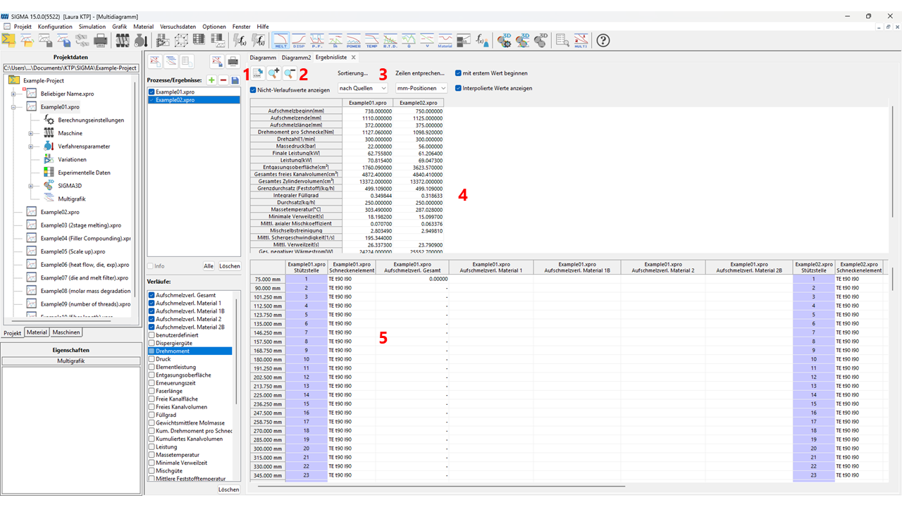
1. Export as .csv File
2. Increase / Decrease Font Size
3. Set Up View
4. Non-Curve Results
5. Curve Results

In the view of the profiles calculated the calculation results can be shown in a table. In the upper part the user can create the view, in the middle part the non-profile-data is shown, and in the lower part the profiles are shown.

The following options are available for the user:

Through deleting the tag the middle part is hidden and there is more space for the profiles.

All profiles from one source (process or results) are sorted side by side. Between the profiles are the positions with blue background. If the profiles are sorted according to profiles from different sources are directly side by side. Therefore it is easier to compare them.

Choosing mm-position the values in the profiles are sorted in a way that the values in a row represent the same mm-position. If a profile has no grid point in this position a corresponding value is linearly interpolated and colored.

Rows represent grid points offers the possibility to compare different values at particular grid points, the mm-positions are in this case displaced.

If the tag is deleted the initial grid points without values are also shown.

Can only be tagged in** Rows represent mm-positions. If **Show interpolated values is tagged in the positions without grid points interpolated values are shown in blue.