The development of a physical-mathematical description of the dispersion process should, based on the present findings, not only be able to describe the deagglomeration process (erosion and rupture) but also the clustering of primary agglomerates. In order to achieve this, the processes were first modelled independently of each other. Subsequently a superimposition was carried out to reach a thorough solution.

In the following considerations, following Bolen and Colwell [BC58], it is assumed that agglomerate disintegration is a process in which a given agglomerate spontaneously breaks down into two parts of equal size under the influence of applied forces. For the disintegration process, in which two parts with a new surface area are formed as shown in the figure, work must be applied to increase the resulting polymer/agglomerate surface area.

Figure: Schematic representation of agglomerate fragmentation

For the work required to increase the surface area, the following applies to this fragmentation process, assuming an isothermal process and a brittle body [BC58] with surface energy $\sigma$:

$$\sigma_M = \frac{\dot{V}_x}{\dot{V}_z}$$

With the change in surface area over time:

$$\overline{\sigma_M} = \frac{\sum_i(\sigma_M L_{Ele})_i}{\sum_i(L_{Ele})_i}$$

the following is obtained for the dispersion efficiency into two spherical particles:

$$P = \frac{\partial W}{\partial t} = 2\sigma\pi d \frac{\partial \bar{d}}{\partial t}$$

According to Rumpf [Rum61], the surface energy is given by:

$$\sigma = \sum_{n=1}^{n_p} \sum_{k=1}^{k} \frac{F_H}{d} = n_p k \frac{\overline{F_H}}{d}$$

Here, $F_H$ denotes the effective adhesive forces, $n_p$ the number of primary particles, and $k$ the number of contact points of the primary particles in the interface to be taken into account.

The minimum power required for a disintegration process is given by:

$$P_{min} = \pi n_p k \overline{F_H} \frac{\partial \bar{d}}{\partial t}$$

In addition to the power, the stresses to which a sphere is subjected in a shear flow are considered in the next step, analogous to [Raa61], [BT74] with regard to the energy input. The particle rotates in the shear flow and is thereby subjected to alternating tensile and compressive stresses. According to Raasch [Raa61], the angular velocity $\omega$ is derived from the prevailing shear velocity of the surrounding flow:

$$\omega = \frac{1}{2} \dot{\gamma} \tag{1}$$

The power at the sphere’s surface, as shown in Figure 10.2, is formulated as follows according to Raasch [Raa61] when considering a pure shear flow:

$$P = \int_{A_{ober}} \left[\sigma_r v_r + \tau_{r\varphi} V_\varphi + \tau_{r\vartheta} V_\vartheta\right] dA$$

The following applies to the surface differential:

$$dA = r^2 \cos \vartheta \, d\vartheta d\varphi$$

Figure: Linear shear flow around a sphere [Raa61]

The stresses arising on the sphere’s surface during the rotation shown about the z-axis are (cf. [Raa61], [HFM92]):

$$\sigma_r = \frac{5}{2} \eta \dot{\gamma} \sin 2\varphi \cos^2 \vartheta$$

$$\tau_{r\varphi} = \frac{5}{2} \eta \dot{\gamma} \cos 2\varphi \cos \vartheta$$

$$\tau_{r\vartheta} = -\frac{5}{2} \eta \dot{\gamma} \sin 2\varphi \sin \vartheta \cos \vartheta$$

The following applies to the velocities:

$$v_r = \frac{\dot{\gamma}}{4} \left(2r - 5\frac{r_0^3}{r^2} + 3\frac{r_0^5}{r^4}\right) \sin 2\varphi \cos^2 \vartheta$$

$$V_\varphi = \frac{\dot{\gamma}}{4}\left[\left(r - \frac{r_0^5}{r^4}\right) \cos 2\varphi - r\right] \cos \vartheta$$

$$V_\vartheta = -\frac{\dot{\gamma}}{4} \left(r - \frac{r_0^5}{r^4}\right) \sin 2\varphi \cos 2\vartheta$$

To calculate the power resulting from the fragmentation process, we now consider the limit at the sphere’s surface for $r = r_0$. The equation then becomes:

$$P = \int_{A_{upper}} \left[\frac{5}{2} \eta \dot{\gamma} \cos 2\varphi \cos \vartheta\right] \left[-\frac{\dot{\gamma}}{2} r_0 \cos \vartheta\right] r_0^2 \cos \vartheta \, d\vartheta d\varphi$$

The figure shows the power distribution on the spherical surface.

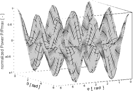
Figure: Power distribution on the spherical surface

For the process of spontaneous disintegration, the shear stress and the maximum value of the power input, as shown in Figure 10.3, are of interest, subject to the boundary condition that $\tau_{r\varphi} = \tau_{crit}$ (critical shear stress, which leads to disintegration when the cohesive forces are exceeded [BT74]), are of interest. The agglomerate is treated here as an isotropic body, so that, regardless of the surface coordinate, exceeding the critical shear stress results in spontaneous disintegration.

The maximum possible shear stress that can occur on the sphere’s surface is given by Eq. (10.16):

$$\tau_{max} = \frac{5}{2} \eta_{Fluid} \dot{\gamma}$$

The circumferential velocity is given by the equation:

$$V_\varphi = r_0 \omega = r_0 \frac{\dot{\gamma}}{2}$$

As a result of these considerations, for a sphere (agglomerate) with diameter $\bar{d}$, the maximum power that can occur is:

$$P_{max} = \frac{5}{4} \eta_{Fluid} \dot{\gamma}^2 \pi r_0^3 = \frac{5}{32} \tau_{Fluid} \dot{\gamma} \pi \bar{d}^3$$

Equating the two power expressions yields the following differential equation:

$$\frac{5}{32} \tau_{Fluid} \dot{\gamma} \pi \bar{d}^3 = 2\pi \cdot n_p k \overline{F_H} \frac{\partial \bar{d}}{\partial t}$$

If we consider the interface of the agglomerate, the number of particles at this interface depends on the surface porosity. The surface porosity $\psi_F$ is calculated according to [PEW93] as the ratio of the area $A_H$ not occupied by the solid to the total area $A$:

$$\psi_F = \frac{A_H}{A} = 1 - \frac{n_p A_p}{A}$$

From this equation, it is possible to derive a relationship for calculating the number of particles in the interface as a function of the surface porosity and the mean agglomerate diameter:

$$n_p = (1 - \psi_F) \frac{A}{A_p} = (1 - \psi_F) \frac{\bar{d}^2}{d_p^2}$$

Substituting the values gives the equation:

$$\frac{5}{32} \tau_{Fluid} \dot{\gamma} \pi \bar{d} = 2(1 - \psi_F) \frac{1}{d_p^2} k \pi \overline{F_H} \frac{\partial \bar{d}}{\partial t}$$

The considerations outlined so far apply to shear fractures in a pure shear flow. However, this does not occur in extruders; rather, in fully filled screw sections, there is always a superposition of compressional and drag flow. Here, the superposition of a pressure gradient in a screw channel results in a shift in the stress state, as shown in Figure 10.4 (Mohr’s stress circle). Accordingly, under sufficiently high pressures, fragmentation can no longer occur under tensile stress. Since experiments have shown agglomerate disintegration particularly in pressurised zones, shear stresses are therefore responsible for the disintegration processes. In partially filled screw sections, too, one is dealing with a multidimensional flow.

Tensile strength, as a material property, may only be used in the case of pure cleavage fractures. For a cleavage fracture perpendicular to the principal tensile stress, the normal stress hypothesis applies. However, this cannot be applied, as pressures significantly higher than the agglomerate strength typically occur in the melt. The extended shear stress hypothesis is appropriate here. It assumes different yield shear stresses. The envelope of the corresponding Mohr’s stress circles is then the yield strength $\tau = f(\sigma)$ [Dub91]. This represents a comprehensive material characteristic. Here, due to incomplete material properties, the envelope is replaced by three straight lines (Figure 10.4).

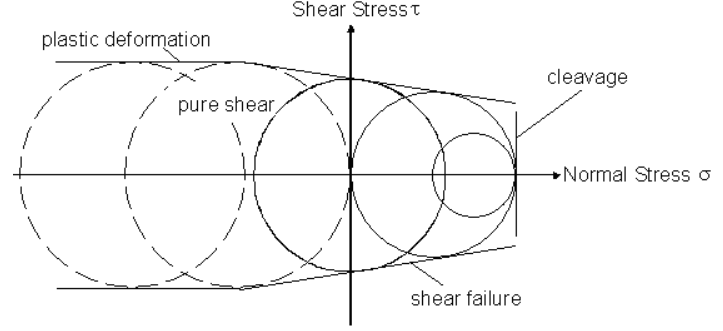
Figure: Limiting agglomerate strength according to Mohr [Dub91]

Due to the high pressures occurring in continuous mixers, shear failures are more than likely to occur. From this follows:

$$\tau_{Sch} = \frac{1}{2} \sigma_v = \sigma_3 - \sigma_1 \tag{10}$$

With σ1 and σ3 being the maximum principle stresses. We assume the hoop stress σv to be almost equal to the tensile strength σz, which we predict using Rumpf's [Rum61] equation:

$$\tau_{Sch} = \frac{1}{2} \sigma_z = \frac{(1 - \varepsilon_A) \overline{F_{adh}}}{2\pi \cdot d_p^2} \tag{11}$$

Inserting the agglomerate strength according to Rumpf (eqn. (11) results in the following differential equation for the agglomerate rupture:

$$\frac{\partial \bar{d}}{\partial t} = \frac{5}{64} \cdot \frac{\tau_{Fluid} \cdot \dot{\gamma}}{\tau_{Sch} \cdot \pi} \cdot \bar{d} \tag{12}$$

Clustering is essentially the collision of particles. In order for particles to collide, two conditions must be satisfied:

1. The particles must move at different velocities.
2. Assuming that all the particles are approximately spherical, the distance between the particles must be smaller than or the same as the sum of their radii.

The following remarks on cluster formation refer to a differential volume element $V$ containing $n_A$ agglomerates.

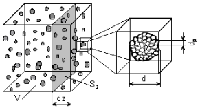
Figure: Differential volume element

Assuming that the agglomerates have similar mean spherical diameters at the same times, a monitoring cross-section can be defined for the agglomeration process, within which agglomerates can come into contact:

$$S_{üb} = \frac{\pi}{4} (d_M + d)^2$$

Figure: Definition of the monitoring cross-section

If we now apply this analysis to a slice of the volume element with length $\partial z$ and cross-sectional area $S_D$, there are $\partial n_A$ agglomerates within this slice:

$$\partial n_A = n_A \frac{S_D \partial z}{V}$$

In relation to the monitoring cross-section, this yields a differential number of agglomerates $n_M$ that may experience a collision:

$$\partial n_M = \frac{\partial n_A S_{mon}}{S_D}$$

Substituting the equations, we obtain:

$$\partial n_M = n_A \frac{\pi (d_M + d)^2}{4 V} \partial z$$

By substituting the solid concentration

$$c_F = \frac{V_F}{V}$$

and the solid volume

$$V_F = n_{A0} V_{A0}$$

we obtain an expression for the rate of change of the number of particles in the volume element:

$$\frac{\partial n_M}{\partial t} = \frac{\partial}{\partial t} \left(\frac{n_A \pi \left(\bar{d}_0 + \bar{d}\right)^2}{n_{A0} 4 V_{A0}} c_F \partial z\right)$$

The number $n_a$ of particles participating in the agglomeration is given by the ratio of the particle volume at time $t > t_0$ to the particle volume at time $t = t_0$:

$$n_a = \frac{\bar{V}_A}{\bar{V}_{A0}} = \frac{\pi \bar{d}^3}{6 \bar{V}_{A0}}$$

Since the essential process in the agglomeration of particles is collision transfer, the change in the number of particles undergoing a collision must be equal to the change in the number of particles participating in the agglomeration. This yields:

$$\frac{\partial n_M}{\partial t} = \frac{\partial n_a}{\partial t}$$

Substituting

$$\frac{\partial n_a}{\partial t} = \frac{\pi 1 \partial \bar{d}^3}{6 \bar{V}_{A0} \partial t}$$

we obtain:

$$\frac{\partial \bar{d}^3}{\partial t} = \frac{3 n_A}{2 n_{A0}} c_F \left(\bar{d}_0 + \bar{d}\right)^2 \frac{\partial z}{\partial t}$$

Since the solid mass in the volume element does not change over time as the agglomerates coalesce, the ratio of the number of particles can be calculated from a mass balance:

$$\frac{n_A}{n_{A0}} = \frac{\bar{d}^3}{\bar{d}_0^3}$$

For two agglomerates to collide, it must also be ensured that there is a relative velocity between the two particles:

$$\bar{v}_{z,rel} = \frac{\partial z}{\partial t}|_{avg} = \frac{1}{2} (v_2 - v_1)$$

If we now derive an expression for the shear velocity of the surrounding fluid

$$\dot{\gamma} = \frac{\partial v_z}{\partial y} = \frac{2(v_2 - v_1)}{(\bar{d}_0 + \bar{d})}$$

and substitute this, we obtain the average relative velocity:

$$\frac{\partial z}{\partial t}|_{avg} = \bar{v}_{z,rel} = \frac{1}{4} \dot{\gamma} (\bar{d} + \bar{d}_0)$$

Substituting gives:

$$\frac{\partial \bar{d}^3}{\partial t} = \frac{1 \bar{d}^3}{8 \bar{d}_0^3} c_F \dot{\gamma} \left(\bar{d}_0 + \bar{d}\right)^2$$

If, analogous to the dispersion analyses by Bolen and Colwell [BC58], it is assumed that only two agglomerates adhere to each other at any one time, the diameter of the agglomerate after cluster formation is given by:

$$\bar{d} = \sqrt[3]{2} \bar{d}_0$$

Finally, introducing the simplification yields the differential equation describing the cluster formation process:

$$\frac{\partial \bar{d}}{\partial t} = \frac{1}{8} \left(1 + \sqrt[3]{2}\right) c_F \dot{\gamma} \bar{d}$$

Which of the three cases discussed above occurs in a given section of a processing machine depends essentially on the shear stress level and the strength of the agglomerates. Three cases must be distinguished here:

• Case 1:
  If the shear stress level is below the critical shear stress for erosion, no deagglomeration will be observed. Agglomerates will clump together. The average agglomerate diameter will increase over time. This case will be observed primarily at very low shear stresses or with agglomerates having very high tensile strength, e.g. due to solid bridges.

• Case 2:
  If the shear stress in the range under consideration lies above the critical shear stress for erosion but below the critical shear stress for fragmentation, it will be observed that individual particles detach from the agglomerate surface. However, no fragmentation of the agglomerates will be observed. The process of erosion is superimposed on the process of cluster formation in this case.

• Case 3:
  If shear stresses exceeding the yield stress for agglomerate break-up are observed, it is to be expected that, on the one hand, the agglomerates will break up and, on the other hand, particles will detach from the agglomerate surface. Here too, it is to be expected that the deagglomeration process is superimposed by an agglomeration process.

A closed-form solution incorporating all three cases can now be obtained from the superposition of the individual processes. If the differential equations describing cluster formation and agglomerate disintegration are superimposed, a differential change in diameter with time results from the sum of the changes in the individual processes:

$$\frac{\partial \bar{d}}{\partial t} = \left(\frac{\partial \bar{d}}{\partial t}\right)_{cluster formation} - \left(\frac{\partial \bar{d}}{\partial t}\right)_{disintegration} - \left(\frac{\partial \bar{d}}{\partial t}\right)_{erosion}$$

To solve the equation, the following dimensionless parameters are defined, which result from the individual processes:

Dimensionless mean agglomerate diameter:

$$d^x = \frac{\bar{d}}{\bar{d}_0}$$

Dimensionless exposure time:

$$t^x = \dot{\gamma} t$$

Disintegration constant:

$$C_{Ze} = \frac{5}{128 \pi}$$ Cluster formation constant:

$$C_{Cl} = \frac{1}{8} \left(1 + \sqrt[3]{2}\right)$$

Erosion constant:

$$C_{Er} = \frac{5}{256 (1 - \psi_F) \pi}$$

Dimensionless stress:

$$\pi_B = \frac{\tau_{Fluid}}{\tau_{Sch}}$$

Applying the dimensionless parameters yields the normalised differential equation:

$$\frac{\partial d^x}{\partial t^x} = C_{Cl} c_F d^x - (C_{Er} + C_{Ze}) \pi_B d^x$$

With the boundary condition that the initial agglomerate diameter

$$d^x (t = t_0 = 0) = 1$$

is, the solution is

$$d^x(t^x) = \exp\{(C_{Cl} c_F - (C_{Er} + C_{Ze}) \pi_B) t^x\}$$

When applying this relationship, the distinction between cases defined above must be taken into account. If the critical shear stresses for erosion or agglomerate fragmentation are not reached during application, the respective dimensionless constants $C_{Ze}$ and $C_{Er}$ in the equations must be set to zero. The limiting shear stresses depend on the specific application (polymer-filler combination) and cannot be specified in general terms [Rum75], [Kre64]. In addition to the yield shear stress, according to Martin [Mar72], a minimum stress duration must be taken into account depending on the specific application, below which no fragmentation can occur even if the yield shear stress is exceeded.

Assuming, analogous to Bolen and Colwell [BC58], that the agglomerate rupture is a process, in which due to imposed hydrodynamic forces an observed agglomerate spontaneously breaks down into two commensurate fractions and assuming furthermore, in simple terms, that agglomerates can be considered spherical, it can be assumed that, given a sufficiently dense packing of the primary particles, the rupture is a planar process. Manas-Zloczower [HFM92] was able to verify this by using computer simulations.

The process of agglomerate rupture involves the creation of new interfaces between the agglomerate fragments and the surrounding polymer (see figure).

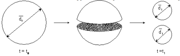
Figure: Schematic diagram of the agglomerate rupture.

The work needed to increase the interface, can generally be defined for this process as:

$$W = \int \sigma dA \tag{1}$$

where σ is the interfacial energy. The power needed to rupture the agglomerates follows from the differentiation of the required rupture work with the time:

$$P = \frac{\partial W}{\partial t} = 2\sigma \pi \bar{d} \frac{\partial \bar{d}}{\partial t} \tag{2}$$

where $\bar{d}$ is the mean agglomerate diameter.

The force necessary for the break down of an agglomerate in this fracture plane, must exceed the sum of the acting adhesion forces.

Equation (3) shall define the interfacial tension as the sum of acting adhesive forces related to the particle diameter analogous to [Rum61]:

$$\sigma = \sum_{n=1}^{n_p} \sum_{k=1}^k \frac{F_{adh}}{\bar{d}} = n_p k \frac{\overline{F_{adh}}}{\bar{d}} \tag{3}$$

with np being the number of primary particles in the fracture plane and k the number of contact points of the primary particles in the fracture plane.

Inserting eqn. (3) into eqn. (2) results therefore in a description of the minimum power required to rupture agglomerates:

$$P_{min} = \pi n_p k \overline{F_{adh}} \frac{\partial \bar{d}}{\partial t} \tag{4}$$

Equating (4) and (13) results in:

$$\frac{5}{32} \cdot \tau_{Fluid} \cdot \dot{\gamma} \cdot \pi \cdot \bar{d}^3 = \pi \cdot n_p k \overline{F_{adh}} \frac{\partial \bar{d}}{\partial t} \tag{5}$$

Looking at the fracture plane of the agglomerate, the number of particles in this fracture plane depends on the area void fraction. The area void fraction εA is, according to [PEW93], calculated as the ratio of the cross-sectional area AV, which is not covered by solids, to the overall cross-sectional area A:

$$\varepsilon_A = \frac{A_V}{A} = 1 - \frac{n_p \cdot A_p}{A} \tag{6}$$

Equation (6) allows the formulation of an equation to calculate the number of particles in the fracture plane which are dependent on the area void fraction:

$$n_p = (1 - \varepsilon_A) \cdot \frac{A}{A_p} = (1 - \varepsilon_A) \cdot \frac{\bar{d}^2}{d_p^2} \tag{7}$$

Inserting (7) in (5) leads to the following equation:

$$\frac{5}{32} \tau_{Fluid} \cdot \dot{\gamma} \cdot \bar{d} = (1 - \varepsilon_A) \cdot \frac{1}{d_p^2} \cdot k \cdot \overline{F_{adh}} \cdot \frac{\partial \bar{d}}{\partial t} \tag{8}$$

The model is so far only valid for cleavages in simple shear flow. Usually the flow in an extruder can not be described using the assumption of a simple shear flow.

The problem is finding a material parameter to describe the strength of an agglomerate. Tensile strengths can only be used for cleavages. For cleavages occurring normal to the principle stress direction, the maximum principle stress criterion can be used. This criterion can not be used here, since the pressures occurring within a continuous mixer are usually greater than the agglomerate strength. We propose to apply Mohr's criterion. It assumes different critical strengths and uses the enveloping lines, Mohr's circles that correspond to the limiting stresses. From this criterion follows:

$$\tau = f(\sigma) \tag{9}$$ [Dub91]

Since there is usually insufficient data, the enveloping lines are replaced by three lines (see figure)

Figure: Limiting agglomerate strength according to Mohr [Dub91]

Due to the high pressures occurring in continuous mixers, shear failures are more than likely to occur. From this follows:

$$\tau_{Sch} = \frac{1}{2} \sigma_v = \sigma_3 - \sigma_1 \tag{10}$$

With σ1 and σ3 being the maximum principle stresses. We assume the hoop stress σv to be almost equal to the tensile strength σz, which we predict using Rumpf's [Rum61] equation:

$$\tau_{Sch} = \frac{1}{2} \sigma_z = \frac{(1 - \varepsilon_A) \overline{F_{adh}}}{2\pi \cdot d_p^2} \tag{11}$$

Inserting the agglomerate strength according to Rumpf (eqn. (11) results in the following differential equation for the agglomerate rupture:

$$\frac{\partial \bar{d}}{\partial t} = \frac{5}{64} \cdot \frac{\tau_{Fluid} \cdot \dot{\gamma}}{\tau_{Sch} \cdot \pi} \cdot \bar{d} \tag{12}$$

In order for primary particles to separate from the agglomerate, the acting shear stresses must overcome the adhesive forces of the primary particles, bonded on the surface of an agglomerate (see figure).

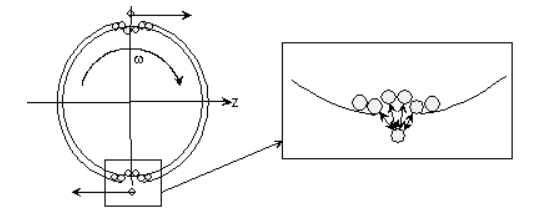
Figure: Schematic diagram of erosion

The work necessary to separate individual particles from an agglomerate, also results from the creation of new surfaces. The minimum power for the observed erosion process can therefore be written as follows:

$$P = \sigma \frac{\partial A}{\partial t} \tag{1}$$

With the surface of an agglomerate consisting of primary particles with the diameter dP:

$$A = n_0 \pi \frac{d_p^2}{2} \tag{2}$$

For the calculation of the number of primary particles n0 on the surface of the agglomerates, it is assumed that the primary particles are evenly distributed over the entire agglomerate and that the void fraction on the surface is the same as the void fraction in any fracture plane [PEW93]:

$$n_0 \pi \frac{d_p^2}{2} \cong (1 - \psi_F) \pi \bar{d}^2 \tag{3}$$

$$n_0 = \frac{2(1 - \psi_F) \bar{d}^2}{d_p^2} \tag{4}$$

It therefore follows for the time-dependent change of the surface of an agglomerate, where particles have been eroded from the outer shell:

$$\frac{\partial A}{\partial t} = \pi (1 - \psi_F) \bar{d} \frac{\partial \bar{d}}{\partial t} \tag{5}$$

The minimum power required to erode particles is calculated using:

$$P_{min} = \sigma \pi (1 - \psi_F) \bar{d} \frac{\partial \bar{d}}{\partial t} \tag{6}$$

The minimum power needed to separate all primary particles from the outer shell of the surface of an agglomerate can therefore be calculated by equating (13) and (6):

$$\frac{5}{32} \tau_{Fluid} \dot{\gamma} \pi \bar{d}^3 = \sigma \pi (1 - \psi_F) \bar{d} \frac{\partial \bar{d}}{\partial t} \tag{7}$$

If, analogous to the rupture, equation (3) is inserted in equation (8), the result is:

$$\frac{5}{32} \tau_{Fluid} \dot{\gamma} \bar{d} = 2n_0 k \overline{F_H} (1 - \psi_F) \frac{\partial \bar{d}}{\partial t} \tag{8}$$

With the number of agglomerates (eqn. 4) the result is:

$$\frac{5}{64} \tau_{Fluid} \dot{\gamma} \bar{d} = 2 \frac{(1 - \psi_F)}{\bar d_p^2} k \overline{F_H} (1 - \psi_F) \frac{\partial \bar{d}}{\partial t} \tag{9}$$

Inserting the defined tensile strength (eqn. 11), according to Rumpf [Rum61], the result is:

$$\frac{\partial \bar{d}}{\partial t} = \frac{5}{256 \pi (1 - \psi_F) \tau_{Sch}} \cdot \tau_{Fluid} \dot{\gamma} \cdot \bar{d} \tag{10}$$

Clustering is essentially the collision of particles. In order for particles to collide, two conditions must be satisfied:

1. The particles must move at different velocities.
2. Assuming that all the particles are approximately spherical, the distance between the particles must be smaller than or the same as the sum of their radii.

Assuming that the agglomerates have similar mean diameters, the second condition mentioned above results in a monitoring cross-section, in which a collision of agglomerates becomes possible (see figure):

$$S_{mon} = \frac{\pi}{4} \left(\bar{d}_M + \bar{d}\right)^2 \tag{1}$$

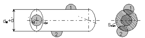
Figure: Definition of the monitoring cross section

For the number of agglomerates ¶nA it is still possible to define the following equation for a differential volume element (see figure):

$$\partial n_A = n_A \cdot \frac{S_D \cdot \partial z}{V} = n_A \cdot \frac{\left(\bar{d}_M - \bar{d}\right)^2}{V} \cdot d_z \tag{2}$$

Related to the monitoring cross section we can get a differential number of agglomerates ¶nM that can experience a collision:

$$\partial n_M = \frac{\partial n_A \cdot S_{mon}}{S_D} = n_A \cdot \frac{\left(\bar{d}_M - \bar{d}\right)^2}{V} \cdot d_z \tag{3}$$

with the solids volume concentration:

$$c_{so} = \frac{V_F}{V} \tag{4}$$

and the total volume of the filler:

$$V_F = n_{A,0} \cdot V_{A,0} \tag{5}$$

We get a description for the change of the differential number of particles experiencing a collision in a differentially small time period ∂t.

$$\frac{\partial n_M}{\partial t} = \frac{\partial n_M}{\partial t} \left(\frac{n_A}{n_{A,0}} \cdot \frac{\pi}{4} \cdot \frac{\left(\bar{d}_M - \bar{d}\right)^2}{V_{A,0}} \cdot c_{so} \cdot \partial z\right) \tag{6}$$

Since the solid matter in the volume element does not change over the time during the clustering of the agglomerates, the ratio of the number of particles can be calculated by means of a mass balance:

$$\frac{n_A}{n_{A,0}} = \frac{\bar{d}^3}{\bar{d}_0^3} \tag{7}$$

The number of particles involved in the clustering process, is derived from the relationship between the particle volume at the time t > to and the particle volume at the time t = to to:

$$n_a = \frac{\nabla_A}{\nabla_{A,0}} = \frac{\pi}{6} \cdot \frac{\bar{d}^3}{\nabla_{A,0}} \tag{8}$$

Differentiating eqn (8) over the time we now reach:

$$\frac{\partial n_a}{\partial t} = \left(\frac{\pi}{6} \cdot \frac{1}{\nabla_{A,0}}\right) \frac{\partial \bar{d}^3}{\partial t} \tag{9}$$

Since the clustering of particles is essentially combined with an impact transmission, the change in the number of particles experiencing a collision in a certain period of time, must be equal to the change in the number of particles involved in the clustering. This leads to:

$$\frac{\partial n_M}{\partial t} = \frac{\partial n_a}{\partial t} \tag{10}$$

Inserting eqn (6) and (9) in (10) we get:

$$\frac{\partial \bar{d}^3}{\partial t} = \frac{3}{2} \cdot \left(\frac{\bar{d}}{\bar{d}_0}\right) \cdot \left(\bar{d} - \bar{d}_0\right) \cdot c_{so} \cdot \frac{\partial z}{\partial t} \tag{11}$$

Where ¶z/¶t is the average relative velocity vz,rel between the agglomerates:

$$\bar{v}_{z,rel} = \frac{2}{\bar{d} + \bar{d}_0} \cdot \frac{0.5(\bar{d}+\bar{d}_0) \cdot 0.5(\bar{d}+\bar{d}_0)}{\int_0^{0.5(\bar{d}+\bar{d}_0)} \dot{\gamma} \cdot dr \cdot dr} = \frac{1}{4} \cdot \dot{\gamma} \cdot (\bar{d} + \bar{d}_0) \tag{12}$$

With eqn. (12) and (11) we get:

$$\frac{\partial \bar{d}^3}{\partial t} = \frac{1}{8} \frac{\bar{d}^3}{\bar{d}_0^3} c_F \dot{\gamma} \left(\bar{d}_0 + \bar{d}\right)^3 \tag{13}$$

Assuming now, analogous to the rupture investigations by Bolen and Colwell [BC58], that two agglomerates will always be clustered, the diameter of the agglomerates after the clustering amounts to:

$$\bar{d} = \sqrt[3]{2} \bar{d}_0 \tag{14}$$

Finally, introducing the simplification in equation (14) into equation (13), results in a differential equation which describes the agglomeration process:

$$\frac{\partial \bar{d}}{\partial t} = \frac{1}{8} \left(1 + \sqrt[3]{2}\right) c_F \dot{\gamma} \bar{d} \tag{15}$$

Which of the three cases discussed above occurs in a given section of a processing machine depends essentially on the shear stress level and the strength of the agglomerates. Three cases must be distinguished here:

• Case 1:
  If the shear stress level is below the critical shear stress for erosion, no deagglomeration will be observed. Agglomerates will clump together. The average agglomerate diameter will increase over time. This case will be observed primarily at very low shear stresses or with agglomerates having very high tensile strength, e.g. due to solid bridges.

• Case 2:
  If the shear stress in the range under consideration lies above the critical shear stress for erosion but below the critical shear stress for fragmentation, it will be observed that individual particles detach from the agglomerate surface. However, no fragmentation of the agglomerates will be observed. The process of erosion is superimposed on the process of cluster formation in this case.

• Case 3:
  If shear stresses exceeding the yield stress for agglomerate break-up are observed, it is to be expected that, on the one hand, the agglomerates will break up and, on the other hand, particles will detach from the agglomerate surface. Here too, it is to be expected that the deagglomeration process is superimposed by an agglomeration process.

A closed-form solution incorporating all three cases can now be obtained from the superposition of the individual processes. If the differential equations describing cluster formation and agglomerate disintegration are superimposed, a differential change in diameter with time results from the sum of the changes in the individual processes:

$$\frac{\partial \bar{d}}{\partial t} = \left(\frac{\partial \bar{d}}{\partial t}\right)_{cluster formation} - \left(\frac{\partial \bar{d}}{\partial t}\right)_{disintegration} - \left(\frac{\partial \bar{d}}{\partial t}\right)_{erosion}$$

To solve the equation, the following dimensionless parameters are defined, which result from the individual processes:

Dimensionless mean agglomerate diameter:

$$d^x = \frac{\bar{d}}{\bar{d}_0}$$

Dimensionless exposure time:

$$t^x = \dot{\gamma} t$$

Disintegration constant:

$$C_{Ze} = \frac{5}{128 \pi}$$ Cluster formation constant:

$$C_{Cl} = \frac{1}{8} \left(1 + \sqrt[3]{2}\right)$$

Erosion constant:

$$C_{Er} = \frac{5}{256 (1 - \psi_F) \pi}$$

Dimensionless stress:

$$\pi_B = \frac{\tau_{Fluid}}{\tau_{Sch}}$$

Applying the dimensionless parameters yields the normalised differential equation:

$$\frac{\partial d^x}{\partial t^x} = C_{Cl} c_F d^x - (C_{Er} + C_{Ze}) \pi_B d^x$$

With the boundary condition that the initial agglomerate diameter

$$d^x (t = t_0 = 0) = 1$$

is, the solution is

$$d^x(t^x) = \exp\{(C_{Cl} c_F - (C_{Er} + C_{Ze}) \pi_B) t^x\}$$

When applying this relationship, the distinction between cases defined above must be taken into account. If the critical shear stresses for erosion or agglomerate fragmentation are not reached during application, the respective dimensionless constants $C_{Ze}$ and $C_{Er}$ in the equations must be set to zero. The limiting shear stresses depend on the specific application (polymer-filler combination) and cannot be specified in general terms [Rum75], [Kre64]. In addition to the yield shear stress, according to Martin [Mar72], a minimum stress duration must be taken into account depending on the specific application, below which no fragmentation can occur even if the yield shear stress is exceeded.

A complete solution, including all three cases, is achieved by a superimposition of the individual processes. The level of shear stress, the residence time and the tensile strength of the agglomerates determine which of the three cases (see above) take place in an designated section of a continuous mixer. The three cases must be distinguished:

• If the observed shear stresses are lower than the critical shear stress for erosion, there will be no deagglomeration. Agglomerates will cluster. The mean agglomerate diameter will increase over time. This will be the case, if the shear stresses are very low or if the tensile strength of the agglomerates is very high.
• If the shear stress in the observed area is higher than the critical shear stress of erosion, but lower than the critical shear stress for rupture, single particles will erode from the agglomerate surface. However, there will be no rupturing of the agglomerate. The erosion process superimposes the clustering process.
• If the shear stress is higher than the critical shear stress for the agglomerate rupture, one can expect that the agglomerates will rupture and that particles will erode from the surface of the agglomerate. Here one can also expect that the deagglomeration process is superimposed by a clustering process.

By superimposing the differential equations for the description of the clustering, erosion and the rupture process, the result is a differential change of the agglomerate diameter over the time as a sum of the diameter changes:

$$\frac{\partial \bar{d}}{\partial t} = \left(\frac{\partial \bar{d}}{\partial t}\right)_{cluster formation} - \left(\frac{\partial \bar{d}}{\partial t}\right)_{dispersive} - \left(\frac{\partial \bar{d}}{\partial t}\right)_{erosion} \tag{1}$$

For the solution of the differential equation, the following dimensionless characteristics, derived from the individual process, are defined as follows:

Dimensionless mean agglomerate diameter:

$$d^x = \frac{\bar{d}}{\bar{d}_0} \tag{2}$$

Dimensionless stress exposure time:

$$t^x = \dot{\gamma} t \tag{3}$$

Rupture constant:

$$C_{Ze} = \frac{5}{128 \pi} \tag{4}$$

Agglomeration constant:

$$C_{Cl} = \frac{1}{8} \left(1 + \sqrt[3]{2}\right) \tag{5}$$

Erosion constant:

$$C_{Er} = \frac{5}{256 (1 - \psi_F) \pi} \tag{6}$$

Dimensionless stress:

$$\pi_B = \frac{\tau_{Fluid}}{\tau_{Sch}} \tag{7}$$

By applying the dimensionless characteristics, the normalized differential equation results in:

$$\frac{\partial d^x}{\partial t^x} = C_{Cl} c_F d^x - (C_{Er} + C_{Ze}) \pi_B d^x \tag{8}$$

Under the boundary condition that the initial agglomerate diameter is:

$$d^x (t = t_0 = 0) = 1 \tag{9}$$

the solution of the differential equation results to:

$$d^x(t^x) = \exp\{(C_{Cl} c_F - (C_{Er} + C_{Ze}) \pi_B) t^x\} \tag{10}$$

For the application of the relationship, the case distinction defined above must be considered. If the critical shear stresses for erosion and agglomerate rupture are not exceeded, the corresponding dimensionless constants (54) and (56) are equal to zero.

The figure shows the dimensionless mean diameter versus the dimensionless stress and the dimensionless exposure time for three different solids volume concentration.

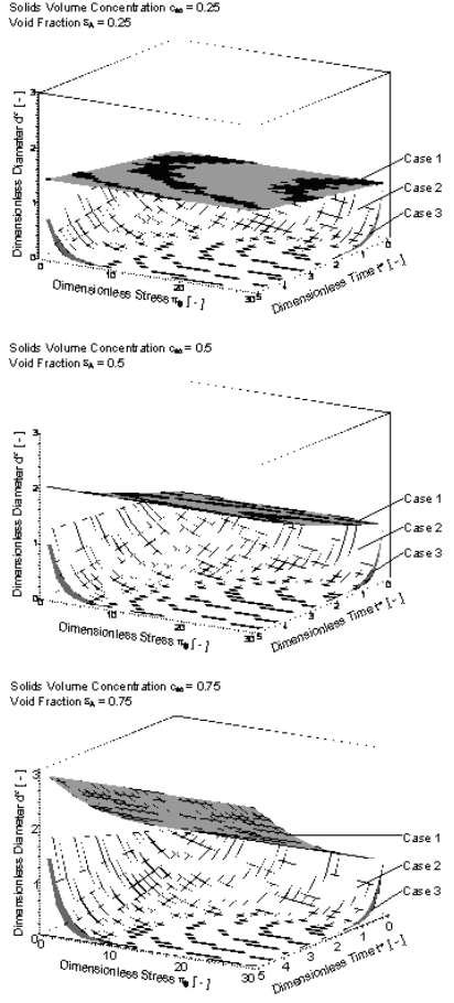
Figure: Dimensionless agglomerate diameter vs. dimensionless time and dimensionless stress for different solid volume concentrations.

When looking at a particular case (see case 1) of the three diagrams, in which no agglomerate dispersion takes place, but the agglomerates form clusters, it becomes evident that the speed, at which the agglomerates form clusters is dependent solely on the solids volume concentration and the stress exposure time.

If there is a shear stress between the critical shear stress for erosion and the critical shear stress for agglomerate rupture, (see case 2), it can be observed that, apart from a dependence upon the dimensionless time and the solids volume concentration, there is also a dependence upon the dimensionless stress.

In the case of shear stresses above the critical shear stress for agglomerate rupture (see case 3), the agglomeration, erosion and rupture processes have to be superimposed to get a the description. Obviously the volume concentration of the solid influences the profile of the dimensionless diameter over the dimensionless time but only if the dimensionless stress is low. While the dimensionless diameter decreases relatively slowly in the case of high solid concentrations, a much more rapid decrease can be observed in the case of low solid volume concentrations.

In order to discuss the results further, it is necessary at this point to define the critical solid volume concentration. Setting $d^*(t^*)=const.=1$ describes the critical solids concentration, at which there is neither an increase nor a decrease in the diameter of the particle.

$$C_{F,krit} = \frac{C_{Er} + C_{Ze}}{C_{Cl}} \pi_B \tag{1}$$

The diagram in the figure shows the critical solids concentration against the dimensionless stress and the agglomerate porosity. The area in which the agglomeration dominates the deagglomeration is situated on the upper side of the plot.

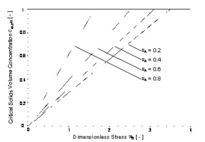
Figure: Critical solid volume concentration vs. dimensionless stress.

Taking into account the different densities of polymers and fillers, the solids weight content is usually considerably higher than the volume content. It can be assumed the agglomerate break down will dominate the agglomerate clustering in most applications. This was taking into account the influence of the area void fraction.

The model describes the effects described in the literature (erosion, agglomerate rupture, agglomerate clustering).

[BC58] Bolen W.R.; Colwell, R.E.: Soc. Plast. Eng. 1958; 14: 24-28

[BT74] Bagster D.F., Tomi, D.: The stresses within a sphere on simple flow fields, Chemical Eng. Science 1974; 29: 1773-1783

[Dub91] Dubbel, Taschenbuch des Maschinenbaus, 1991

[HFM92] Horwatt, S., Feke, D., Manas-Zlocyower, I.: The influence of structural heterogeneities on the cohesivity and breakup of agglomerates in simple shear flow, Powder Technology 1992; 72: 113-119

[Kre64] Krekel J.: Herstellung und Messung von Scherströmungen mit extrem großer Schubspannung und ihr Einfluss auf die Zerkleinerung von Agglomeraten, 1964

[Mar72] Martin G.: Untersuchung der Homogenisierfunktion von Einschneckenextrudern für die Kunststoffverarbeitung, 1972

[Pah89] Pahl MH.: Lagern, Fördern und Dosieren von Schüttgütern, Verlag TÜV Rheinland, 1989

[Raa61] Raasch J.: Beanspruchung und Verhalten suspendierter Festsstoffteilchen in Scherströmungen hoher Zähigkeit, 1961

[Rum61] Rumpf H.: Agglomeration, Intern. Symposium Philadelphia 1961: 379-418

[Rum75] Rumpf H.: Mechanische Verfahrenstechnik, München, Wien: Carl Hanser Verlag, 1975