Torque and Power Consumption
Original Model
The total power consumption is made up of solid friction and mixing friction in the feeding section, the power in the intermeshing zone of both screws, the power in the radial clearance over the screw tips, the power in the melt layer between solid material and the barrel wall, the power in the melt pool and in the melt section. In the calculation of the processes, the power consumption is considered to be negligibly tiny until the place of the first melt pool formation. As co-rotating twin screws, which will be used as a plasticating unit, usually possess a partly filled feeding zone, this is justifiable.
In the estimation of the power consumption in [KSS81] equations were represented, where the power is calculable in the general form:
$$P = \int_0^z \int_{-\frac{b_{max}}{2}}^{+\frac{b_{max}}{2}} (\tau_{0x} r_{0x} + \tau_{0z} r_{0z}) dx \, dz \tag{1}$$
With the wall shear stress:
$$\tau_{0x} = K \left[\left(\frac{\partial v_x}{\partial y}\right)^2 + \left(\frac{\partial v_z}{\partial y}\right)^2\right]^{\frac{n-1}{2}} \frac{\partial v_x}{\partial y} \tag{2}$$
$$\tau_{0z} = K \left[\left(\frac{\partial v_x}{\partial y}\right)^2 + \left(\frac{\partial v_z}{\partial y}\right)^2\right]^{\frac{n-1}{2}} \frac{\partial v_z}{\partial y} \bigg|_{y=h} \tag{3}$$
if the shear rates at the wall for conveying elements with the represented approximation equations in the table are used.
Table: Estimation of the wall shear speeds (conveying elements: [KSS81])
| I., III. | II. |
|---|---|
| $ \left.\frac{\partial v_x}{\partial }\right|_{y=h} = \frac{v_{0x}}{h}\,C_x $ | $ \left.\frac{\partial v_x}{\partial y}\right|_{y=h} = \frac{v_0}{h}\,C_x $ |
| $ \left.\frac{\partial v_z}{\partial }\right|_{y=h} = \frac{v_{0z}}{h}\,C_z $ | $ \left.\frac{\partial v_z}{\partial y}\right|_{y=h} = \frac{v_0}{h}\,C_z $ |
I. Conveying Elements
$$C_x = \left[(1.368 + 2.634n^{0.1})e^{(n-1)^{\frac{1}{n}}}\right]\tag{4}$$
$$0.55 \leq \pi_V \leq 1.00 \quad\quad C_z = 1 + 3n^{-0.2131}(1 - \pi_V)\tag{5}$$
$$1.00 < \pi_V \leq 1.25 \quad\quad C_z = 1 + 3(1 - \pi_V)\tag{6}$$
$$1.25 < \pi_V \leq 2.00 \quad\quad C_z = C_1 - C_2 \pi_V^{C_3}\tag{7}$$
II. Kneading Blocks
$$C_x = \frac{1}{\pi} + \sqrt{2}\tag{8}$$
$$C_z = \frac{\pi + 1}{\pi} \cdot \frac{\dot{V}}{v_0 b_{max} h k}\tag{9}$$
III. Reconveying Elements
$$C_x = 1.75 + 1.75n\tag{10}$$
$$0.00 \leq \pi_V \leq 1.00 \quad\quad C_z = (0.42 + 0.8828n)\pi_V + (1.75 + 1.9692n)\tag{11}$$
For re-conveying elements, the two equations shown in table can be used. These approximation equations are based on a numerical solution of a system of differential equations, the systems of differential equations table [KSS81]. The same prerequisites are used as were for the equations of the conveying elements [KSS81].
The estimation of the power consumption must differ in the 3 function sections in the figure on the barrel wall and in the melting section.
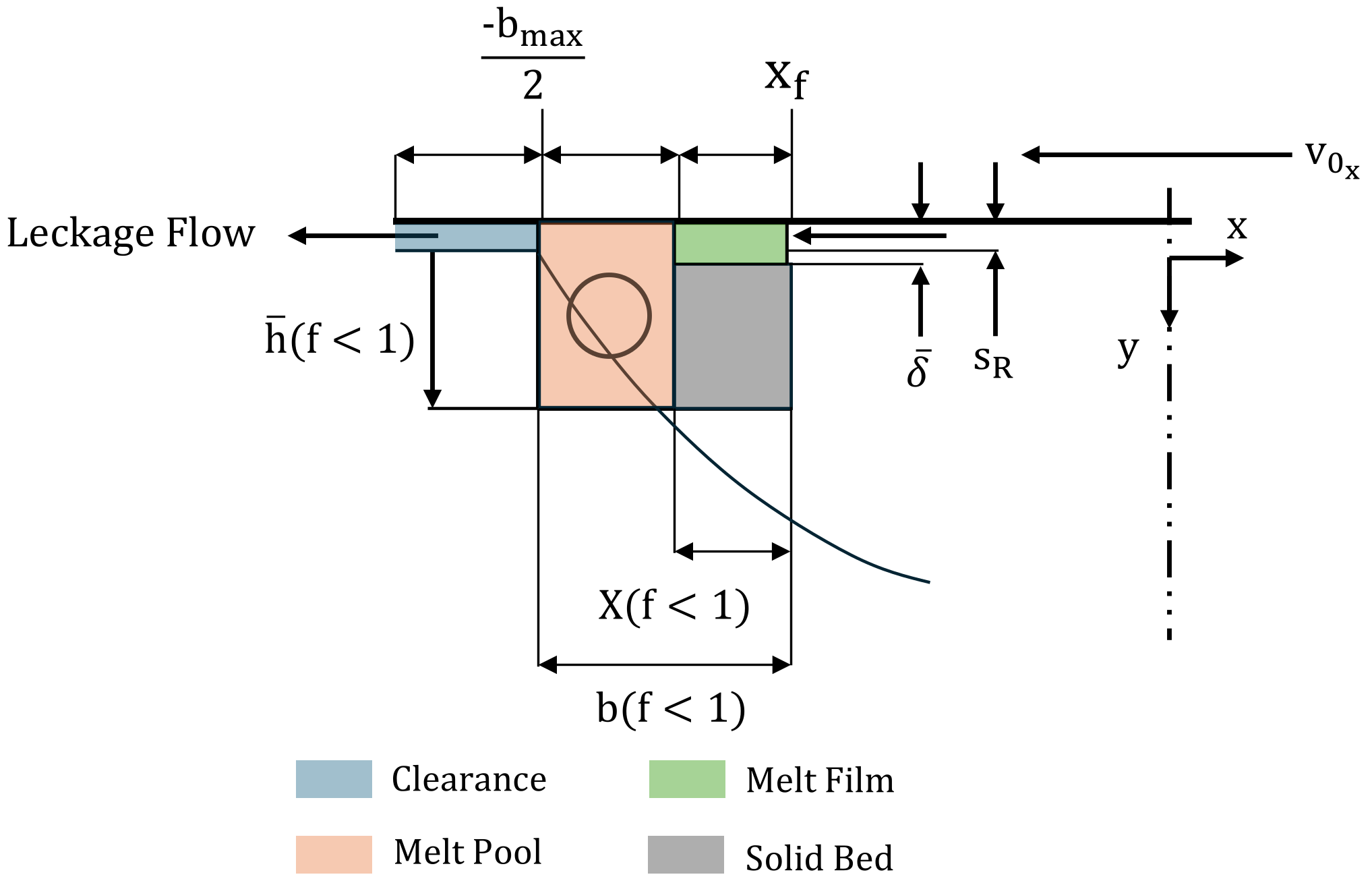
Figure: Model for the power calculation.
The calculation of the power consumption within each section is explained hereafter (for conveying elements and kneading blocks).
Melting Range
The power consumption can be calculated in zones of constant geometry using the following equation:
$$P_1 = \left\{\int_0^{l_n} \left[C_z^2 + \tan^2(\varphi_s) C_x^2\right]^{\frac{1}{2}} C_z + v_{0x}^{l_n} \left[C_z^2 \cot^2(\theta_G) + C_x\right] + C_x \right\} \frac{|k(T)b(1-y)\Delta z_k}{h} \tag{12}$$
Depending on the value of y a pure melt section, consider equation (1) (y = 0) a melt pool in the melting section (0 < y < 1).
In addition the radial clearance is considered through:
$$P_2 = \frac{K(T_Z)e_{max}\Delta z v_{0z}^{1+n}}{s_R^n} \{1 + \tan^2(\varphi_s)\}^{\frac{n+1}{2}} k \tag{13}$$
Equation (2) assumes a pure drag flow over the radial clearance.
Melting Section
According to the figure the melting section is divided up into two areas:
Melt film on the barrel wall with an underlying solid bed of the width: $b \cdot y$
The principle is again the same as that in equation
$$P = \int_0^z \int_{-\frac{b_{max}}{2}}^{+\frac{b_{max}}{2}} (\tau_{0x} r_{0x} + \tau_{0z} r_{0z}) dx \, dz\tag{14}$$
For the melt film, the shear stresses are to be replaced according to [For87] as follows:
$$\tau_{0x} = K(T_{Fl}) \left(\frac{v_{rel}}{\delta}\right)^{n-1} \frac{v_{0x}}{\delta} \tag{15}$$
$$\tau_{0z} = K(T_{Fl}) \left(\frac{v_{rel}}{\delta}\right)^{n-1} \frac{v_{0z} - v_{Fz}}{\delta} \tag{16}$$
With this the relative speed of the melt film $v_{rel}$ will be formed using:
$$v_{rel} = \sqrt{(v_{0z} + v_{Fz})^2 + v_{0x}^2} \tag{17}$$
This results in the consumption:
$$P_3 = \frac{K(T_{Fl}) \overline by\Delta z v_{rel}^{n-1}}{n} (v_{0x}^2 + (v_{0z} - v_{Fz})v_{0z})k \tag{18}$$
A prerequisite of this way of modelling is the assumption of a pure drag flow in the melt film.
Melt Layer
Depending on the value of y, bearing in mind equation
$$P_1 = \left\{v_{0z}^{1+n} \left[C_z^2 + \tan^2(\varphi_s) C_x^2\right]^{\frac{n-1}{2}} C_z + v_{0x}^{1+n} \left[C_z^2 + \cot^2(\varphi_z) + C_x\right]^{\frac{n-1}{2}} C_x\right\} \frac{K(T_{Fl})b(1-y)\Delta z}{n} k\tag{19}$$
a pure melt section ($y = 0$) or a melt pool in the melting section ($0 < y < 1$).
The individual powers in the different function ranges and zones yield the power consumption in the processing unit of the machine.
$$P = \sum(P_1)_i + \sum(P_2)_i + \sum(P_3)_i \tag{20}$$
The specific energy yield is a frequently used parameter for the interpretation of a processing unit. It is calculated by using the ratio of power consumption to mass flow:
$$S_{Ve} = \frac{P}{\dot{m}} \tag{21}$$
And it is proportional to the product: $\overline{\eta \dot{\gamma}^2} t$, respectively proportional to the product: $\overline{\tau \dot{\gamma}} t$.
The screw torque yields from the total power consumption using the:
$$M_d = \frac{P_{total}}{4n_D x} \tag{22}$$
The screw torque is related to that of one screw.
Modified Model
Estimation of the Power Consumption
The starting point for the energetic examination is an energy balance at an extruder (see figure).
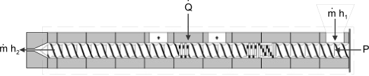
Figure: Energy balance at a co-rotating twin screw extruder.
The drive power P of the screw in combination with the heat exchanged at the barrel wall generates an enthalpy increase of the extruded material (open, stationary system). The mathematic formulation of the energy balance reads as follows:
$$\dot{P} + \dot{Q} = \dot{m} \cdot (h_2 - h_1) = \dot{m} \cdot \Delta h \tag{23}$$
The total screw performance divides in the screw channel into the dissipation and the pressure build-up (see figure). The fraction of kinetic energy can be neglected, however [TK78], [TG79]:
$$P = P_{Diss} + P_{Vol} = P_{Diss} + \Delta p \cdot \dot{V} \tag{24}$$
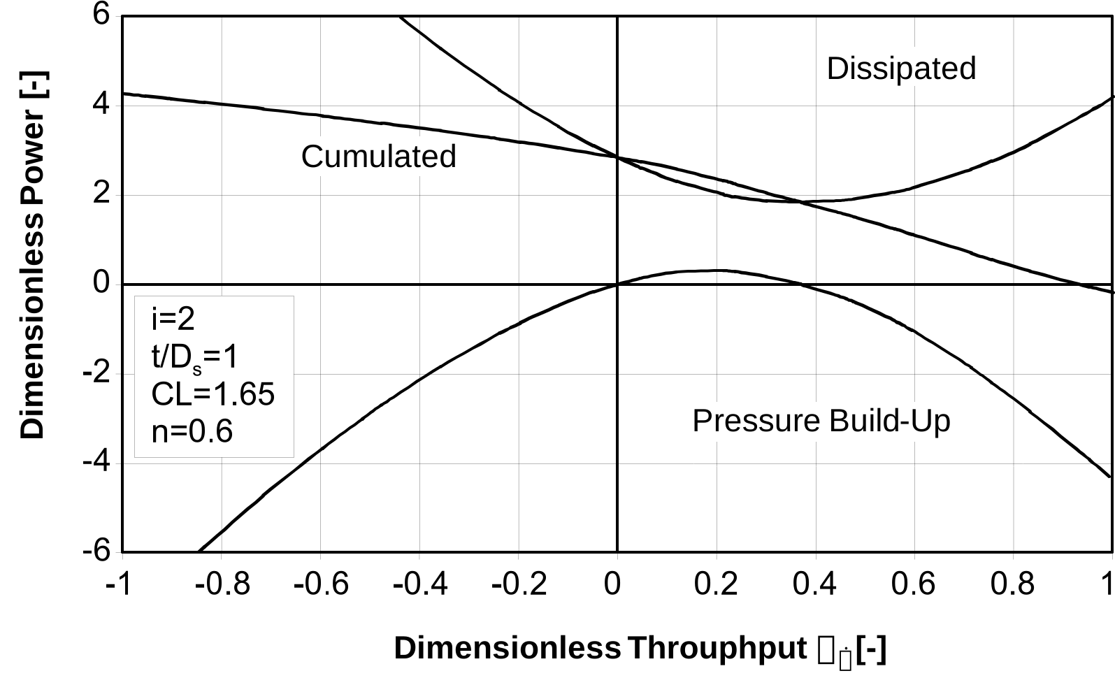
Figure: Power fractions in dependence on the dimensionless volume throughput.
For the modeling of the power input some simplifying assumptions are made as follows:
- The melt is wall-adhering.
- The flow be stationary, incompressible and laminar creeping (c=cv=cp).
- All material values, except the viscosity, are considered as being temperature invariant.
- The flow properties of the melt comply with the Power Law: $\tau = K \cdot \dot{\gamma}^n$
In the calculation of the required drive power a global distinction has to be made according to the functional zones of the extruder and a local distinction according to the zones in the screw elements. In the following the solids conveying zone, the homogenizing section and the zone of pure melt transport will be understood as the basic functional zones. Mixing sections for the incorporation of fillers or for the blend of polymers will not be examined separately here, however.
In contrast to the extraction of solid materials in co-rotating twin screw extruders the extraction in single screw extruders is not dominated by drag mechanisms but by forced conveying mechanisms. For this reason, the power input is negligible in the solids feed zone of a co-rotating twin screw extruder as compared to the other zones [Mel98].
Power Input in the Melt Transport Zone
Volumetric Strain Energy
The Volumetric strain energy is defined as a product of pressure difference and volume flow.
$$P_{Vol} = \Delta p \cdot \dot{V} \tag{25}$$
Is Equation 25 standardized the following equations result for the single geometries:
- Twin screw channel
$$\pi_{Pow.Vol.DSE} = \frac{\Delta p \cdot \dot{V}}{\Delta z} \cdot \frac{\bar{h}^n}{K \cdot b_{max} \cdot v_0^{1+n}} = \pi_{p.DSE} \cdot \pi_{\dot V.DSE} \tag{26}$$
- Rectangular channel
$$\pi_{Pow.Vol.RE} = \frac{\Delta p \cdot \dot{V}}{\Delta z} \cdot \frac{h^n}{K \cdot b \cdot v_0^{1+n}} = \pi_{p.RE} \cdot \pi_{\dot V.RE} \tag{27}$$
- Disk element
$$\pi_{Pow.Vol.SE} = \frac{\Delta p \cdot \dot{V}}{L} \cdot \frac{1}{K \cdot A_{free} \cdot n_0^{n+1}} = \pi_{p.SE} \cdot \pi_{\dot V.SE} \tag{28}$$
The calculation is performed on the basis of the models introduced in chapter 3 of [Kre04]. In the figure the variations predicted by means of the model are contrasted with the results of the flow simulation. A sufficient description of the volumetric strain energy can be recognized for the whole area.
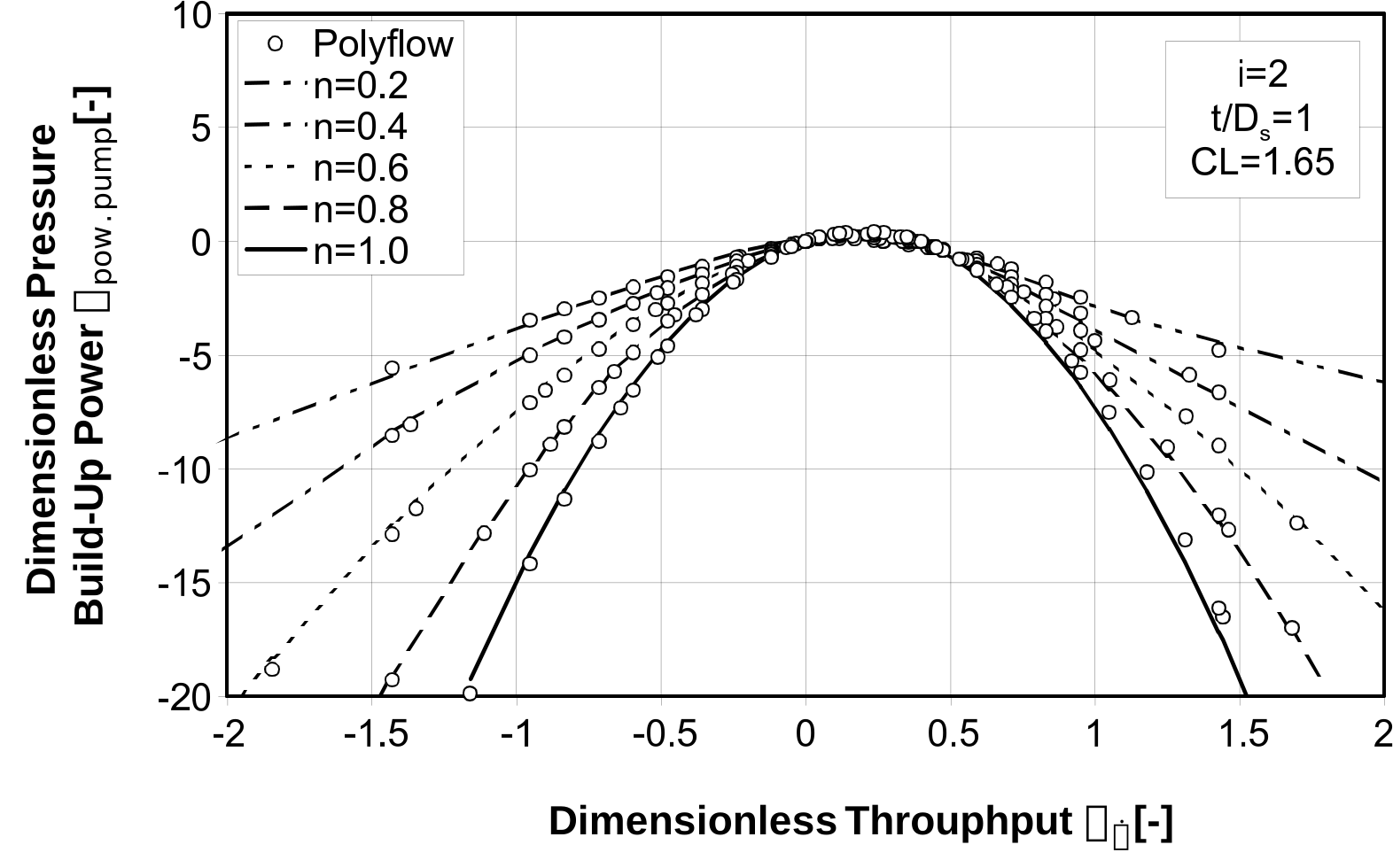
Figure: Dimensionless pumping capacity in dependence of the dimensionless volume throughput.
Dissipated Energy
In the context of the evaluation of the flow simulations the dissipated energy in the flow-channels was also determined. For this purpose, the locally dissipated energies were determined in every volume element of the channel and subsequently integrated over the whole channel (Eq. 29):
$$P_{diss} = \int \tau \cdot \dot{\gamma} \cdot dV = \sum_{i=1}^n \eta_i \cdot \dot{\gamma}_i^2 \cdot V_i \tag{29}$$
Before modeling the dissipated energy the values determined by means of Equation 29 were standardized. In the table the dimensionless parameters are presented for the examined geometries.
With the assistance of regression analyses specification approaches were developed, with which the dissipated energies in rectangular channels, twin screw channels and disk elements can be predicted.
Dimensionless parameters for the specification of the dissipated energy:
- Rectangular channel:
$$\pi_{Pow.Diss.RE} = \frac{\Delta P_{Diss.RE}}{\Delta z} \cdot \frac{h^n}{K \cdot b \cdot v_0^{1+n}}\tag{30}$$
- Twin screw channel:
$$\pi_{Pow.Diss.DSE} = \frac{\Delta P_{Diss.DSE}}{\Delta z} \cdot \frac{\bar{h}^n}{K \cdot b_{max} \cdot v_0^{1+n}}\tag{31}$$
- Disk element:
$$\pi_{Pow.Diss.SE} = \frac{\Delta P_{Diss.SE}}{L} \cdot \frac{1}{K \cdot D_s^2 \cdot n_0^{n+1}}\tag{32}$$
- Rectangular channels
$$\pi_{Pow,Diss,RE} = C_{Pow,RE,0} + C_{Pow,RE,1} \cdot \pi_{\dot{V},RE} + C_{Pow,RE,2} \cdot \pi_{\dot{V},RE}^2 + C_{Pow,RE,3} \cdot \pi_{\dot{V},RE}^3 + C_{Pow,RE,4} \cdot \pi_{\dot{V},RE}^4 \tag{33}$$
- Twin screw channels
$$\pi_{Pow,Diss,DSE} = C_{Pow,DSE,0} + C_{Pow,DSE,1} \cdot \pi_{\dot{V},DSE} + C_{Pow,DSE,2} \cdot \pi_{\dot{V},DSE}^2 + C_{Pow,DSE,3} \cdot \pi_{\dot{V},DSE}^3 + C_{Pow,DSE,4} \cdot \pi_{\dot{V},DSE}^4 \tag{34}$$
- Disk elements
$$\pi_{Pow,Diss,SE} = C_{Pow,SE,0} + C_{Pow,SE,1} \cdot \pi_{\dot{V},SE}^{1.5} \tag{35}$$
The figure displays the comparative relation of the dissipated energies calculated with the Polyflow and the model predictions for a twin screw channel.
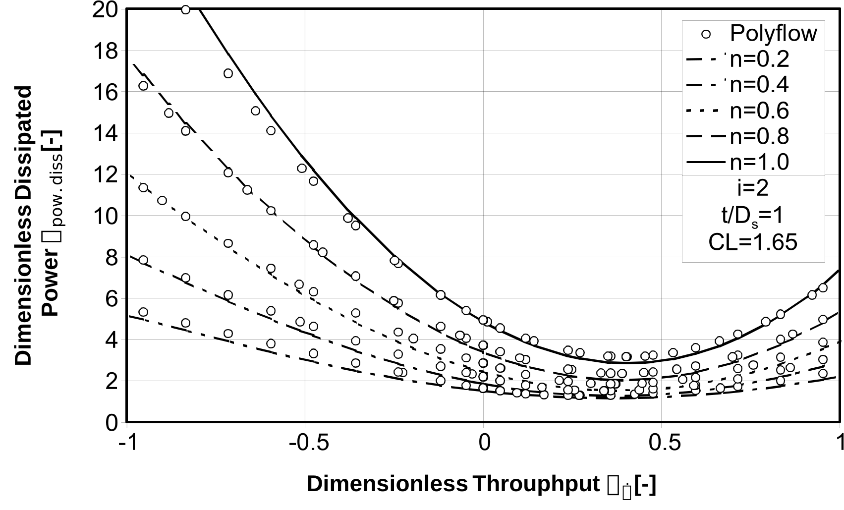
Figure: Comparison of the model predictions and the dissipated energies calculated with Polyflow for a twin screw channel.
A satisfactory accordance is observed here also. The parameters in the equations 33 to 35 depend on the geometry and the material data, i.e. on the exponent of the Power Law. The estimation of the parameters can be found in detail in the appendices C1.2, C2.2 and C3.2 in [Kre04].
Estimation of the Power Input in the Screw Elements
For the estimation of the power input in the screw elements the energy fractions (dissipation and volume change) and the separate areas in the screw elements are superposed. In Table the equations for the estimation of the power in the different mixing elements are enlisted.
Power of the screw elements
| Element Type | Power Equation |
|---|---|
| Thread element | $P_{GE} = P_{Diss.channel} + \Delta p_z \cdot \dot{V}_z + P_{Diss.gap} + \Delta p_x \cdot \dot{V}_x$ |
| Closely intermeshing thread mixing element | $P_{dGME} = P_{Diss.channel} + \Delta p_z \cdot \dot{V}_z + P_{Diss.gap} + \Delta p_x \cdot \dot{V}_x + P_{Diss.groove} + \Delta p_N \cdot \dot{V}_N$ |
| Non-intermeshing thread mixing element | $P_{tGME} = P_{Diss.channel.fe} + \Delta p_{z.fe} \cdot \dot{V}_{z.fe} + P_{Diss.gap.fe} + \Delta p_{x.fe} \cdot \dot{V}_{x.fe} + P_{Diss.groove.fe} + \Delta p_{N.fe} \cdot \dot{V}_{N.fe} + P_{Diss.channel.fe} + \Delta p_{z.fe} \cdot \dot{V}_{z.fe} + P_{Diss.gap.fe} + \Delta p_{x.fe} \cdot \dot{V}_{x.fe} + P_{Diss.groove.fe} + \Delta p_{N.fe} \cdot \dot{V}_{N.fe}$ |
| Toothed mixing element | $P_{TME} = P_{Diss.disc} + \Delta p_{SE} \cdot \dot{V}_{SE} + P_{Diss.groove} + \Delta p_N \cdot \dot{V}_N$ |
For the verification of the model experiments were performed with a laboratory extruder. Silicon oil of the Baysilone 50.000 type was utilized as experimental medium. For the measurement of the power the drive unit of the extruder was suspended in an oscillating way and the section modulus was measured by means of a spring-balance, which was attached to a lever arm. Deriving from the measurement of the section modulus and the screw speed as well as the knowledge of the transmission gear ratio the drive power could thus be determined. The figure displays a comparison of the measured dimensionless drive power and the dimensionless drive power calculated with the model for closely intermeshing thread-mixing elements. The accordance is good, particularly by considering the simplifications made in the modeling.
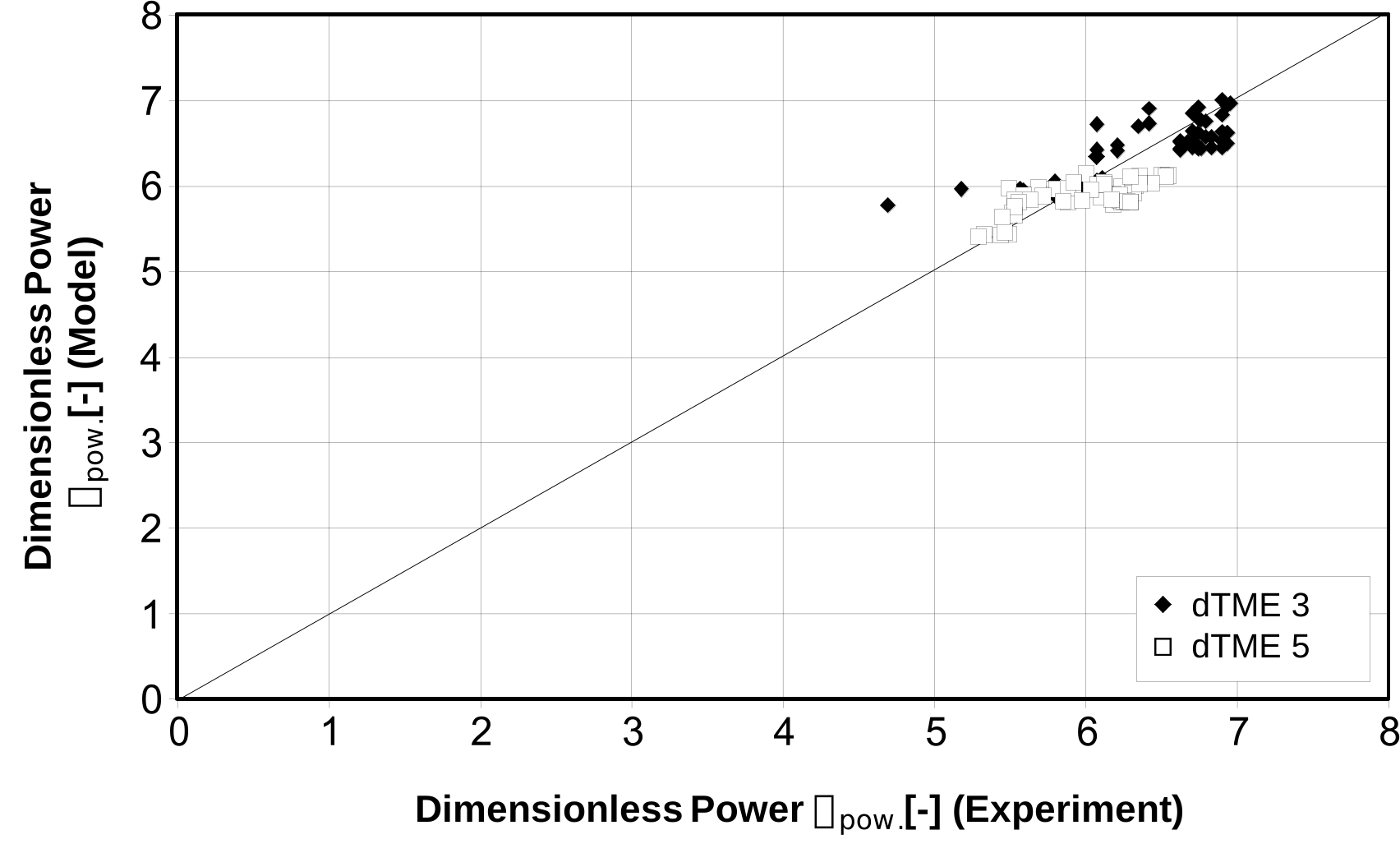
Figure: Comparison of the measured and the calculated dimensionless drive power for closely intermeshing thread-mixing elements.
Estimation of the Power Input in Partly-filled Screw Zones
Co-rotating twin screw extruders are operated in a regulated form, i.e. the extruder is impressed with a mass flow rate, independent of the conveying capacity of the applied screw elements. Resulting from this, the extruder is partly filled over a wide area. Whether a partial filling can be observed at a specific mass flow rate, essentially depends on the applied material, the operating point and the geometry of the separate screw elements. As some of those screw and mixing elements concerned here can be partly filled (with the only exception of neutral and back-flow toothed mixing elements and non-intermeshing thread mixing elements), the estimation of the drive power in the partly filled sections is also important for mixing elements, even if in practice the operating point is usually arranged in such a way that a partial filling of these elements does not arise.
The approach to calculate the power input at partial fillings will be demonstrated by considering a thread element as example, but can be transferred in an analogous manner to all mixing elements examined in this piece of work.
In case of a partial filling a pressure gradient cannot emerge, so that the equation for the estimation of the drive power in thread elements (see table) simplifies to:
$$P_{GE} = P_{Diss.channel.tf} + P_{Diss.gap} \tag{36}$$
It is simplifyingly assumed that the radial clearance is completely loaded and that a pure drag flow prevails here. For the estimation of the energy dissipation in the partly filled channel the following equation applies:
$$P_{Diss.channel.tf} = f \cdot P_{Diss.channel.vf} \tag{37}$$
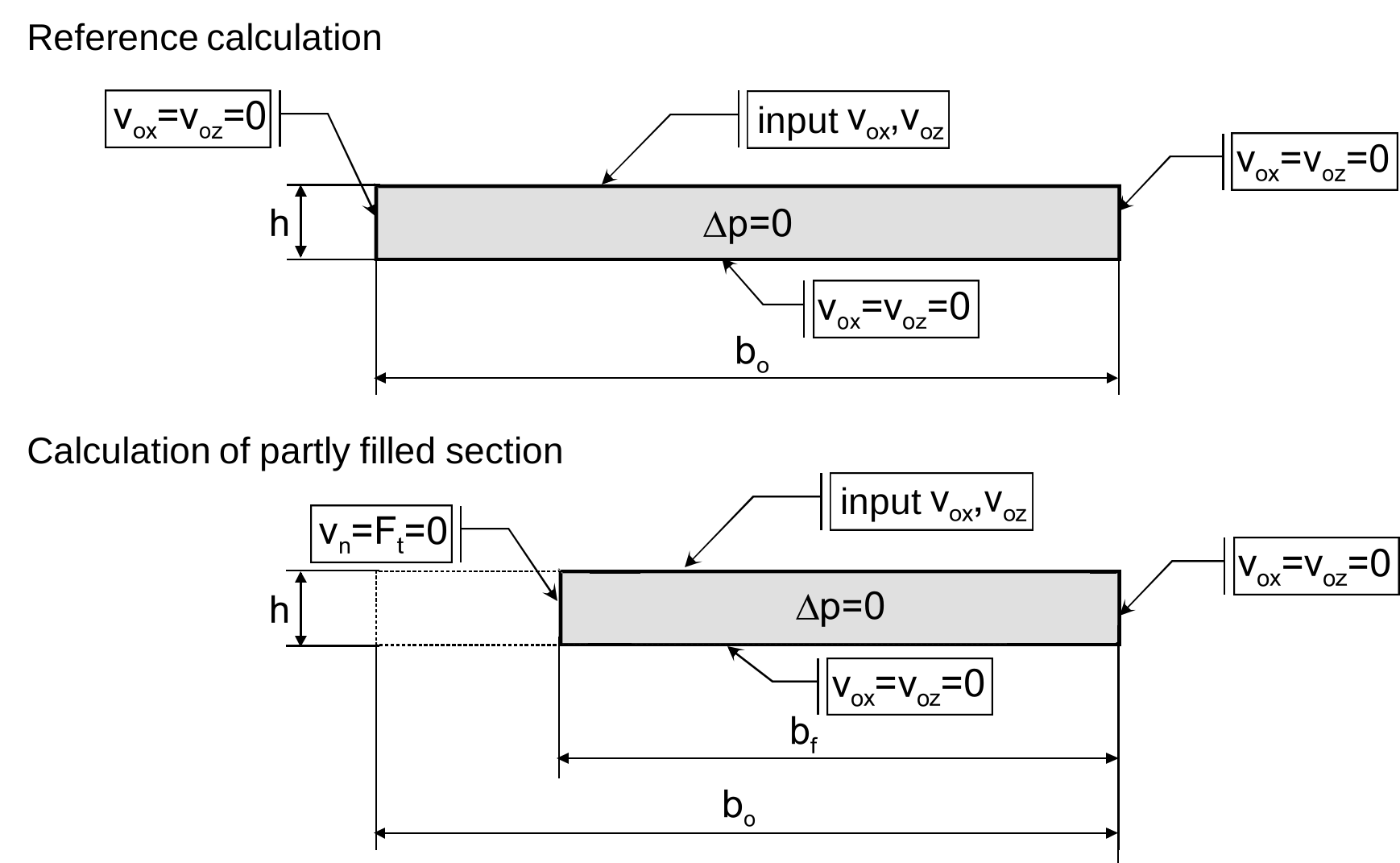
Figure: Boundary conditions for the simplified simulation of a partly filled screw section.
For the verification of this equation exemplary finite element simulations were performed with the boundary conditions as illustrated in the figure. The starting point of the simulations was a fully loaded rectangular channel with a ratio of channel height to channel width of b/h=40. For the exemplary simulations of party filled channels the depth of the reference channel is reduced. Additionally, the boundary conditions are then also changing for the simulation at the rear face of the flight, which represents the open area. In contrast to the reference computation at this area non-negligible velocities are defined; it is predetermined that at this area tangential forces do not emerge. In all cases the dissipated energy and the shear rate were calculated.
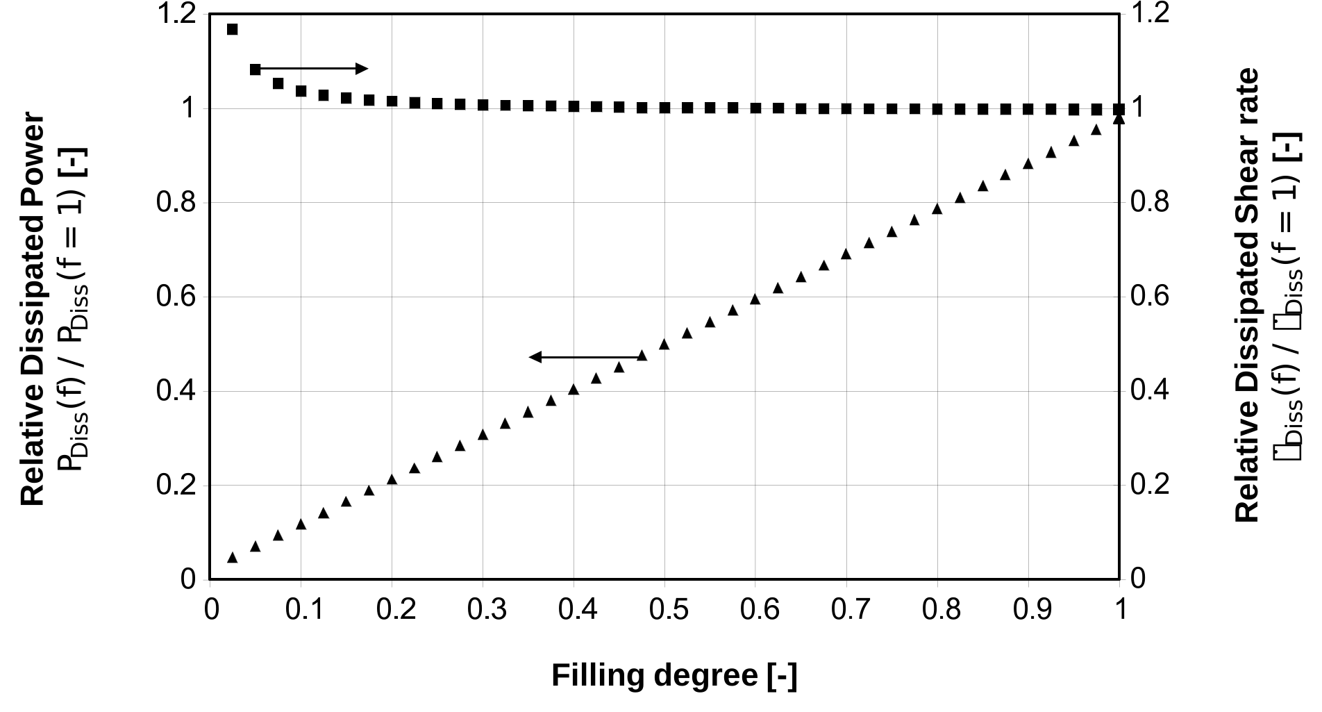
Figure: Dependence of the relative dissipated energy and the relative shear rate on the loading content.
The figure illustrates the relative dissipated energy in dependence of the loading content. It can be recognized that the interrelationship presented in Equation 37 is affirmed. A slight deviation can be observed, however, which results from the different boundary conditions of the simulation. Furthermore, it is remarkable that the medium shear rate proves constant over a wide scope of loading contents. Due to the boundary effects a deviation can be noticed only at low loading contents (f < 0.2). These findings do not conform with the estimation approaches for the shear rate published by Ansahl [Ans93] and Melisch [Mel98], which act on the assumption that the medium shear rate accelerates continuously at loading contents, which are lower than 1.
Torque calculation
In the area of the solids conveying zone, it is assumed that relatively little energy is introduced into the plastic. The energy input and the applied torque of the zone are negligible.
In the melting zone, the power applied to melt and transport the plastic is converted into the torque required for this. Assuming that the melting is dominated by the plastic deformation of the granulate and not by the heat input via the barrel wall, the energy required for this comes from the screw shafts.
The torque per screw is calculated here by:
$$M_d = \frac{ \frac{P}{n \cdot 2 \cdot \pi}}{2}\tag{38}$$
Once a melting degree of 100% has been reached, the energy introduced is based on the conveying and mixing of the plastic. The torque generated here can be calculated using a lever arm and the force applied. The lever arm is determined as a function of the filling level and the element geometry from the difference between the screw radius and the channel depth at the point where the force is applied (x).
$$l(x) = \frac{D_s}{2} \left(1 - \left[1 + \cos\left(\frac{2 \cdot \pi \cdot \left(|x| - \frac{e_{max}}{2}\right)}{t \cdot \cos(\varphi_s)}\right)\right] - \sqrt{a_{th}^2 - \frac{D_s^2}{2} \cdot \sin^2\left(\frac{2 \cdot \pi \cdot \left(|x| - \frac{e_{max}}{2}\right)}{t \cdot \cos(\varphi_s)}\right)}\right)\tag{39}$$
The shear stresses acting on the element surface result from the existing shear rates and the local viscosity.
$$\begin{bmatrix} \frac{dv_x}{d_x} & \frac{dv_x}{d_y} & \frac{dv_x}{d_z} \\ \frac{dv_y}{d_x} & \frac{dv_y}{d_y} & \frac{dv_y}{d_z} \\ \frac{dv_z}{d_x} & \frac{dv_z}{d_y} & \frac{dv_z}{d_z} \end{bmatrix} \cdot \eta = \begin{bmatrix} \sigma_x & \tau_{xy} & \tau_{xz} \\ \tau_{yx} & \sigma_y & \tau_{yz} \\ \tau_{zx} & \tau_{zy} & \sigma_z \end{bmatrix}\tag{40}$$
A laminar flow is assumed as a boundary condition, which means that there is no flow from the screw to the cylinder and therefore no shear rate in the y-direction over the channel height and width.
$$\frac{dv_y}{d_x}, \frac{dv_y}{d_z} = 0\tag{41}$$
In partially filled areas, the normal forces can be disregarded.
The shear stresses are related to the projected areas of the duct floor, the duct surface and the duct wall.
$$\begin{bmatrix} \sigma_x & \tau_{xy} & \tau_{xz} \\ \tau_{yx} & \sigma_y & \tau_{yz} \\ \tau_{zx} & \tau_{zy} & \sigma_z \end{bmatrix} \cdot \begin{bmatrix} A_{Wand} \\ A_{Boden} \\ A_{Kanal} \end{bmatrix} = \begin{bmatrix} F_x \\ F_y \\ F_z \end{bmatrix}\tag{42}$$
Using the same procedure, a torque component is calculated for the gap between the screw and barrel and these are added together.
The energy input results from:
$$P_{spez. mech.} = \frac{M_d \cdot n \cdot 2 \cdot \pi}{\dot{m}}\tag{43}$$
The new model is activated in the calculation settings by ticking the checkbox for torque consideration.
Enthalpy Model
Power calculation via enthalpy
In order to guarantee the three goals of improving accuracy, reducing complexity and considering all process zones in the new power model, a model approach was developed using the first law of thermodynamics. To understand the modelling of the model, the enthalpy input into the polymer is shown formulaically in the three process zones, solids conveying zone, melting zone and melt zone.
Solids conveying zone
First of all, a specific enthalpy curve of a semi-crystalline plastic is considered (Picture 1). At the crystallite melting temperature, the plastic has a corresponding specific enthalpy depending on the type. This enthalpy is divided in PAM into $\Delta h_f$ solid enthalpy (enthalpy change to increase the solid temperature) and $\Delta h_a$ melting enthalpy (enthalpy required to dissolve the crystalline regions).
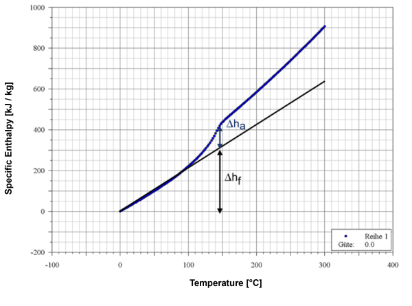
Picture 1: Specific enthalpy curve of a partially crystalline polymer
The specific enthalpy change at a supporting point compared to the filling point of the material results from the multiplication of the solid enthalpy by a percentage factor which is dependent on the filling temperature, the current solid temperature and the crystallite melting temperature. The factor indicates to what percentage of the crystallite melting temperature the solid was heated, starting from the starting temperature of the material. The melting enthalpy is initially not taken into account in the solids conveying zone. The reason is shown in figure 1. For the determination of the enthalpy increase must be referred to the black imaginary straight lines. If the melting enthalpy is taken into account, the straight line would have a too large gradient at low temperatures, resulting in too large a deviation. In the solids conveying range, however, the temperature increase lies precisely in this small value range. Formally expressed, the specific enthalpy change at a support point in the solids conveying range compared to the filling point is given by equation 44:
$$\Delta h_{FF} = \Delta h_f \cdot \frac{T_{FS} - T_E}{T_K - 0}\tag{44}$$
For the driving power of an element area the difference of the specific enthalpy change between two supporting points is calculated with equation 45.
$$\Delta \Delta h_{FF} = \Delta h_{FF_n} - \Delta h_{FF_{n-1}}\tag{45}$$
Using the calculated specific enthalpy difference, the pressure difference and the introduced heat flow, the required drive power required between two support points in the solids transport zone can be calculated from this (46).
$$P_{D/FF} = \dot{m} \ast (\Delta \Delta h_{FF} + \frac{\Delta p}{\rho}) - \dot{Q}\tag{46}$$
Melting zone and melt conveying zone
The melting zone and the melt conveying zone differ from the solids conveying zone in that the material is two-phase. Consequently, a separate consideration of the specific enthalpy change must be carried out for the solids bed and the melt zone.
For the specific enthalpy change of a pure heating of the melt, the following applies in relation to the crystallite melting temperature through the integration of the specific heat capacity via the temperature equation 47.
$$\Delta h_{RS} = cp_0 \ast (T_M - T_K) + \frac{m_{cp}}{2} \ast (T_M^2 - T_K^2)\tag{47}$$
In addition to the enthalpy, energy was already introduced into the molten material by heating the melt in order to heat the solid up to the crystallite melting temperature. Formally, the specific enthalpy introduced up to the melting point can be determined according to equation 44 with equation 48.
$$\Delta h_{FA} = \Delta h_a + \Delta h_f \ast \frac{T_K - T_E}{T_K - 0}\tag{48}$$
From the addition of the equations 47 and 48, equation 49 results for the specific enthalpy increase from the starting point of the filling temperature to the current melt temperature for the melt range:
$$\Delta h_S = \Delta h_a + \Delta h_f \ast \frac{T_K - T_E}{T_K - 0} + cp_0 \ast (T_M - T_K) + \frac{cp_m}{2} \ast (T_M^2 - T_K^2)\tag{49}$$
The solid bed in the melting zone, on the other hand, undergoes a different specific enthalpy increase. This can be determined with equation 44, following equation 50 in the solids conveying area.
$$\Delta h_{FA} = \Delta h_f \ast \frac{T_{FS} - T_E}{T_K - 0}\tag{50}$$
The enthalpy increases of the solid bed and the melt zone must now be weighted and added up on the basis of the degree of melting in order to obtain the total enthalpy change at a supporting point in the melting zone and the melt conveying zone. For weighting, the total mass flow is multiplied by the respective percentage of the solid or melt. By adding the two specific enthalpy changes, the total enthalpy increase at one support point can be calculated. The differentiation between melting zone and melt area is made by the degree of melting. This is calculated in advance in SIGMA and can also be displayed in visual form.
In the pure melt conveying zone, for example, the melting degree is equal to one, so that the second term of equation 51 is omitted.
$$\Delta h_{AS/S} = m_{asv} \ast \Delta h_S + (1 - m_{asv}) \ast \Delta h_{FA}\tag{51}$$
The required driving power of an element area can be determined with the available results via the difference of the specific enthalpy increase of two supporting points (equation 51) via equation 52.
$$\Delta \Delta h_{AS/S} = \Delta h_{AS/S_n} - \Delta h_{AS/S_{n-1}}\tag{52}$$
$$P_{D_{AS/S}} = \dot{m} \ast (\Delta \Delta h_{AS/S} + \frac{\Delta p}{\rho}) - \dot{Q}\tag{53}$$
Power calculation of a single-stage compounding process
In the single-stage compounding process, two polymers are metered into the hopper and then compounded. This means that the components are dosed in a certain ratio in the hopper and simultaneously plasticized. As a result, both materials have the same temperature at one point along the extrusion process. However, the polymers differ in their melting behaviour. At the same temperature, both materials also have different enthalpy levels. The consequence is that the components mixed in the hopper cannot be seen as a unit, but that the enthalpy levels must be considered separately and then added, weighted, to the corresponding mass flow. The advantage of this method is that the model is not only applicable for two polymers, but for any number of them. In addition, the basic model already modelled can be used and only a weighting and addition of both enthalpy levels is required.
In the solids transport zone, the enthalpy level of the individual polymers can be calculated using equation 44. These are then weighted with equation 54 and added together to obtain the enthalpy level at a supporting point.
$$\Delta h_{FF_{C1}} = \frac{\dot{m}_1}{\dot{m}_{SS}} \ast \Delta h_{FF1} + \frac{\dot{m}_2}{\dot{m}_{SS}} \ast \Delta h_{FF2} + \cdots + \frac{\dot{m}_n}{\dot{m}_{SS}} \ast \Delta h_{FFn}\tag{54}$$
Subsequently, identical to equation 45 and equation 46, the enthalpy change and from this the required drive power between two adjacent support points can be calculated.
The same method is used in the melting zone and the melt conveying zone. The enthalpy levels of the polymers are considered separately in the first step and then added together. Equations 49 and 50 of the basic model provide the enthalpy levels of the corresponding melt and solid content for the individual polymers. In equation 51 the proportions are weighted with the enthalpy level. For a process with several polymers that melt simultaneously, the weighting of the different mass flows must also be taken into account. Equation 55 applies to the specific change in the enthalpy when compounding polymers when mixed in the hopper:
$$\Delta h_{AS/S_{C1}} = \frac{\dot{m}_1}{\dot{m}_{SS}} \left(\dot{m}_1 \ast m_{asv_1} \ast \Delta h_{S_1} + \dot{m}_1 \ast (1 - m_{asv_1}) \ast \Delta h_{FA_1}\right) + \frac{\dot{m}_2}{\dot{m}_{SS}} \left(\dot{m}_2 \ast m_{asv_2} \ast \Delta h_{S_2} + \dot{m}_2 \ast (1 - m_{asv_2}) \ast \Delta h_{FA_2}\right)$$ $$ + \cdots + \frac{\dot{m}_n}{\dot{m}_{SS}} \left(\dot{m}_n \ast m_{asv_n} \ast \Delta h_{S_n} + \dot{m}_n \ast (1 - m_{asv_n}) \ast \Delta h_{FA_n}\right)\tag{55}$$
Subsequently, identical to equation 52 and equation 53, the specific enthalpy difference and the required drive power between two supporting points can be calculated.
Power calculation for a two-stage compounding process
At the beginning of the process, first one material is plasticized and later in the direction of extrusion two or more materials are plasticized simultaneously. As a result, different numbers of polymers are present at different support points in the extrusion process, which determine the enthalpy level. For this reason, the process must be regarded as a separate application. For the modelling of a two-stage process, it is again possible to fall back on the models already created. Before the calculation, however, a case distinction must be made to check whether one or more polymers are processed in the extruder. Up to the second material stage, the enthalpy increase compared to the filling temperature can be calculated strictly according to the basic model from chapter 5. If a support point meets an additional material stage or material addition, the model from the single-stage compounding process must be used. Please note that the individual mass flows are not related to the total mass flow of all polymers, but only to the mass flow of the current support point.
Power model for the compounding of fillers
During compounding, fillers such as chalk or talcum are often incorporated to change material properties. For this purpose, the fillers are added to the plasticized melt. A modification of the models presented in this paper is not necessary. However, two cases are to be considered critically. In the case of extremely high filler contents, additional power is required due to the newly generated frictional forces. However, these are special processes and will not be considered at first. The second critical case is the support point where the fillers are incorporated. Through the addition, the melt experiences a significant reduction in temperature. The consequence is that the enthalpy difference with the previous supporting point becomes negative. As a result, the total power requirement between the two support points becomes less than zero. This process is physically impossible because theoretically no power can be obtained from the extruder. The solution is to set the power requirement at this point to zero. This is acceptable because conveying elements are used at the filler addition point, which generally have a low power requirement.
Power model for a melt extruder
In the melt extruder, the specific increase in enthalpy due to melting of the solid is eliminated. The melt conveyed in the extruder only undergoes a change in enthalpy due to a temperature variation. For this reason, the calculation of the enthalpy increase up to the melting point can be neglected and the reference point for the enthalpy change is not the filling temperature but the crystallite melting temperature. With later differentiation of the enthalpy changes this portion would be shortened out again anyway. The specific enthalpy change of a melt at a support point in the melt extruder in relation to the crystallite melting temperature can be calculated using Equation 49 with Equation 56.
$$\Delta h_{SE} = cp_0 \ast (T_M - T_K) + \frac{cp_m}{2} \ast (T_M^2 - T_K^2)\tag{56}$$
For the driving power, the difference of the specific enthalpies is calculated again (57):
$$\Delta \Delta h_{SE} = \Delta h_{SE_n} - \Delta h_{SE_{n-1}}\tag{57}$$
Equation 58 applies to the drive power:
$$P_{D_{SE}} = \dot{m} \ast (\Delta \Delta h_{SE} + \frac{\Delta p}{\rho}) - \dot{Q}\tag{58}$$
Power model for a melt extruder with several polymers
In the case of a twin-screw extruder, which functions as a melt extruder and is equipped with a melt consisting of several polymers, the model must be modified for a melt extruder. The procedure is similar to that for compounding. The individual enthalpy levels of the components are determined in a first step and then weighted with the aid of the mass flows. Formally, equation 59 is obtained.
$$\Delta h_{SE_M} = \frac{\dot{m}_1}{\dot{m}_{ges}} \left(cp_{01} \ast (T_M - T_K) + \frac{cp_{m1}}{2} \ast (T_M^2 - T_K^2)\right) + \frac{\dot{m}_2}{\dot{m}_{ges}} \left(cp_{02} \ast (T_M - T_K) + \frac{cp_{m2}}{2} \ast (T_M^2 - T_K^2)\right) $$ $$+ \cdots + \frac{\dot{m}_n}{\dot{m}_{ges}} \left(cp_{0n} \ast (T_M - T_K) + \frac{cp_{mn}}{2} \ast (T_M^2 - T_K^2)\right)\tag{59}$$
Subsequently, as in the case of a melt extruder, which is loaded with a polymer, the difference of the enthalpy change can be formed and from this the drive power between two support points.
Total drive power
With the relationships shown, the individual required drive powers between two support points or the individual elements can be determined and visualized in SIGMA. Finally, the individual calculated element powers must be added up to obtain the total power. The sole consideration or difference of the initial and final enthalpy to determine the power leads to errors in various cases. This is the case, for example, if the melt temperature drops once during the extrusion process due to fillers and the melt is then heated again. The subsequent heating of the melt must be done by new energy from outside. This requires a further input of power, which would be neglected if the initial and final enthalpy were simply compared.
Enthalpy model with heat flow
The enthalpy model neglects the heat flow between the polymer and the barrel wall. While in larger industrial extruders the proportion of heating power to total power is small compared to the drive power, neglecting the heat flow can lead to significant errors, particularly in smaller laboratory extruders or processes with a large temperature difference between the melt and the barrel.
To account for the heat flow, the heat transfer coefficient is calculated according to [TM00]. First, the Brinkmann number is calculated and then the Nusselt number is regressed from it.
$$Br=\frac{K*v_{0}^{n+1}}{\lambda*\Delta T*h^{n-1}}\tag{60}$$
$$Nu=2,9*Br^{0,8}\tag{61}$$
The heat transfer coefficient can then be calculated using the thermal conductivity of the melt and the channel height:
$$\alpha=\frac{Nu*\lambda}{h}\tag{62}$$
The heat flow is calculated as follows:
$$\dot Q=\alpha*l_{Node}*U_{Barrel}*\frac{b_{eff}}{b_{max}}*\Delta T\tag{63}$$
The heat flow is subtracted from the calculated specific enthalpy difference according to equation 46 in order to determine the corrected drive power. This calculation is performed when the 'Enthalpy w. heat flow' power model is selected.
Validation
The new power model was implemented and verified in SIGMA. Identical to other models, the new power model was compared with the values of the experimental investigations to validate the model. The deviations of different process points and material combinations are shown in the following picture.
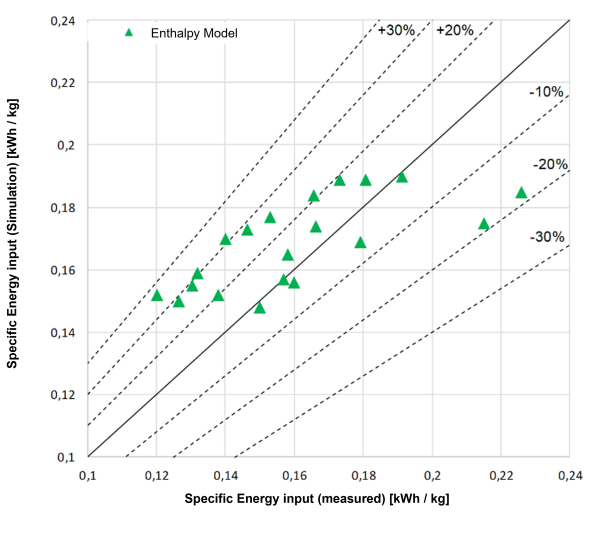
Figure: Comparison of experimental investigations and simulations
References
[Ans93] Ansahl, J.: Grundlagen für die Auslegung dichtkämmender Gleichdrall-Doppelschneckenextruder, Dissertation Universität Paderborn, 1993
[For87] Fornefeld, A.: Approximationsgleichungen zur Auslegung von Mehrzonen-Plastifiziereinheiten mit Scher- und Mischelementen, Dissertation, Universität Paderborn, 1987
[Kre04] Kretschmer, K.: Untersuchung und Beschreibung des Prozess- und Mischverhaltens von Mischelementen für Gleichdrall-Doppelschneckenextruder, Dissertation, Universität Paderborn, 2004
[KSS81] Kim, W.-S.; Skatschkow, W.-W.; Stungur, J.W.: Experimentelle und theoretische Untersuchungen der Durchsatz-Druck-Kennlinien von Doppelschneckenextrudern, Plaste und Kautschuk, 28(1981)2, 93-100
[Mel98] Melisch, U.: Grundlagen zur Simulation des Förder- und Plastifizierprozesses dichtkämmender Gleichdrall-Doppelschneckenextruder; Dissertation; Universität Paderborn; 1998
[TG79] Tadmor, Z.; Gogos, C.: Principles of Polymer Processing, John Wiley & Sons, Brisbane, Chichester, Toronto, 1979
[TK78] Tadmor, Z.; Klein, I: Engineering Principles of Plasticating Extrusion, Robert E. Krieger Publishing Company, Huntington, New York, 1978
[TM00] Tenge, S.; Mewes, D.: “Experimental investigation of the energy balance for the metering zone of a twin screw extruder”; Polymer Engineering & Science; Volume 40; 2000; S. 277–289