Dies ist eine alte Version des Dokuments!
Fiber Fracture Calculation
Basic Considerations
For the following considerations of the modeling of the glass fiber reduction during compounding at first the real geometry is transferred into an unwind channel model. The channel model is kinematically reversed, so that the flow processes can be described under the following assumptions:
- Laminar, stationary flow
- High viscosity melt
- Flow behavior is described by the power law.
Following [Ans93] and [Mel98] a shear flow can be assumed in the channel and in the radial gap areas in partly-filled screw zones. In fully-filled areas the flow conditions result from a superposition of the shear flow and the pressure flow. The radial gap regions are dominated by only a shear flow.
On the basis of this point of view it can be expected that the fibers in the polymer matrix orient with the shear flow. The fibers are thus forced by with the surrounding polymer. It is assumed that the shear stress on the fiber in the channel area will not be enough to cause the fibers to break. The shear stress in the intermeshing zone and above the radial gaps - in contrast to that in the channel area - is several times higher and thus in these areas the flow stress will be high enough to cause the fibers to break.
These preliminary considerations are the basis for the following modeling steps.
Modeling
For modeling the glass fiber reduction, preliminary tests have been taken into account. At these preliminary tests a screw geometry consisting of a pre-distributor kneading block and screw mixing elements is used for the incorporation (see Figure 1).
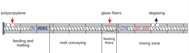
Figure 1: Screw geometry preliminary tests
Dead-stop experiments with varying screw speed, throughput and pressure at the screw tip have been conducted with a constant glass fiber amount. Thus, melt samples could be taken along the incorporation zone and be measured with regard to the glass fiber length.
These tests showed that the profiles of the average glass fiber length along the mixing zone show an exponential decrease. This profile is qualitatively shown in Figure 2.

Figure 2: Qualitative profile of the glass fiber length
For a description of this behavior the following differential equation is used:
$$\frac{dl}{dt} = c \cdot l^{\infty} ; \text{with} l = \frac{L - L_{\infty}}{L_0 - L_{\infty}} \tag{1}$$
The origin of this equation refers to the initial glass fiber length $L_0$ with a dimensionless fiber length $l$, which describes the relation of the current glass fiber length $L$ to the initial fiber length $L_0$. The equation profile asymptotically approaches a process-limited fiber length $L_{\infty}$. The further parameters describe the speed $c$ and the sensitivity $α$ in terms of a fiber breakage.
Process-limited Fiber Length
For a solution of this differential equation and in particular for determining the process-limited fiber length $L_{\infty}$ the preliminary considerations about flow processes in twin-screw extruders are used.

Figure 3: Shear flow stress on a fiber
The first approach is that the fiber is going to break in the center and the fiber-fiber interaction will be neglected. A single fiber in the shear flow is forced by the shear stress $\tau$ (see Figure 3) that acts at its generated surface. The resulting force can be written as:
$$\tau = \frac{F_{flow}}{A_{surface}} \Rightarrow F_{flow} = \tau \cdot A_{surface} \tag{2}$$
In case that the fiber is stopped by a barrier, like somewhere in the gap or in the intermeshing region, the ratio of the critical compressive force, coming from Euler buckling (see Figure 4), to the resulting force from the flow decides if the fiber is going to break or not. The critical compressive force is defined as follows
$$F_{kink} = \frac{\pi^2 \cdot E \cdot I}{L^2} \tag{3}$$
Here $E$ is the fiber-Young's-modulus, $I$ the minimal moment of inertia of the fiber and $L$ the fiber length [BG97].

Figure 4: Euler buckling
If the force from the flow dominates the critical compressive force, the fiber will break in the centre. In the next step half of the fiber length is regarded. If the ratio of these forces is still bigger than one, the fiber will again break in the centre. This procedure will go on until the ratio is smaller than one, so that the critical compressive force dominates the force from the flow and the process-limited fiber length is found. This approach shows that the final fiber length basically depends on the shear stress in the system and the fiber geometry. This procedure is illustrated in the following figure.

Figure 5: Calculation process for the final fiber length
Determining the Sensitivity α
The surrounding of the flow creates a constant force per length on the fiber. The resulting bending line $w(x)$ (see Figure 6) can be expressed in:
$$w\left(\frac{x}{L}\right) = \frac{F \cdot L^2}{48 \cdot E \cdot I} \left(3 \cdot \frac{x}{L} - 4 \cdot \left(\frac{x}{L}\right)^2\right) \tag{4}$$

Figure 6: Resulting bending line at stressed fiber
In the middle of the fiber is the maximum bending load. The maximum bending moment $M(x)$ follows in dependence of the second derivative of the bending line $w''$:
$$M\left(\frac{x}{L}\right) = -E \cdot I \cdot w'' ; max. M\left(\frac{1}{2}\right) = \frac{F}{L} \cdot \frac{L^2}{12} \tag{5}$$
The load of tension depends on the bending moment and it is proportional to the fiber length l squared:
$$\sigma = \frac{M}{I} \cdot \frac{D}{2} \sim L^2 \tag{6}$$
In Equation 6 $D$ is the fiber diameter.
The tensile strength $R_m$ is a material parameter and independent of the fiber length itself:
$$R_m \sim L^0 \tag{7}$$
The parameter α can be described by the ratio of the load of tension to the tensile strength of the fiber. It follows:
$$sensitivity = \frac{tension strain}{strength} \sim L^2 ; \alpha = 2 \tag{8}$$
Solving the Differential Equation
With the determined sensitivity the following is true for Equation 1:
$$\frac{dl}{dt} = c \cdot l^2 ; \text{with } l = \frac{L - L_{\infty}}{L_0 - L_{\infty}} \tag{9}$$
In this case the solution for the equation depending on the time $t$ is:
$$I(t) = -\frac{1}{c \cdot t + k} \tag{10}$$
The constant k can be calculated with the initial condition:
$$I(t = 0) = -\frac{1}{c \cdot 0 + k} = 1 \tag{11}$$
$$\Rightarrow k = -1 $$
With the following boundary condition the speed $c$ which is connected with the fiber breakage can be calculated:
$$I(t = t_0) = -\frac{1}{c \cdot t_0 - 1} = \frac{1}{2} \tag{12}$$
$$\Rightarrow c = \frac{1}{t_0}$$
The time constant $t_0$ corresponds in this case to the time after which the fiber breaks in the middle.
$$I(t) = -\frac{1}{\frac{t}{t_0} + 1} \tag{13}$$
The time constant $t_0$ refers to the process-related residence time $t_V$.
Estimating the Time Constant t₀
With assuming that the dissipated work is a factor for the probability of fracture, it is related to the energy that leads to a fiber breakage.
For the flow energy the following is valid:
$$E_{diss} = \tau \cdot A \cdot v \cdot t_V \tag{14}$$
The product from shear stress, the surrounding area $A$, velocity of the melt v and residence time tV are then transformed to:
$$E_{diss} = \overline{ \eta \dot{\gamma}^2} \cdot V \cdot t_V \tag{15}$$
Here $\eta$ is the viscosity, $\dot{\gamma}$ the shear rate, $V$ the volume of the considered channel section and $t_V$ the residence time.
A consideration of the fiber leads to the following for the fracture energy:
$$E_{breakage} = n \cdot \int F dS \tag{16}$$
The force $F$ per length $S$ related to n fibers in the system forms the fracture energy. If the force $F$ is expressed by the product from the fracture stress $σ$ and the fibre cross sectional area, the following is true for the fracture energy:
$$E_{breakage} = n \cdot \frac{\pi \cdot D^2}{4} \cdot L \cdot \int_0^{\varepsilon_0} \sigma d\varepsilon \tag{17}$$
The solution of the integral and a transformation of the geometry of the fibers lead to:
$$E_{breakage} = V \cdot \Phi \cdot \frac{E \cdot \varepsilon_B}{2} \tag{18}$$
The volume $V$ of n fibers in the system is described by the volume of the considered channel section related to the fiber volume ratio $\Phi$. The Young's Modulus and the elongation at break $ε_B$ of the fiber characterize the fracture stress.
As soon as the flow energy is higher than the fracture energy, the fiber will break. Balancing both forms of energy as follows:
$$\frac{E_{diss}}{E_{breakage}} = \frac{2 \cdot \eta \cdot \dot{\gamma}^2}{\Phi \cdot E \cdot \varepsilon_B} \cdot t = 1 \tag{19}$$
means the following for the time constant $t_0$:
$$t_0 = \frac{\Phi \cdot E \cdot \varepsilon_B}{2 \cdot \eta \cdot \dot{\gamma}^2} \tag{20}$$
In this case the time $t$ corresponds to time constant $t_0$ after which the fiber broke in the middle. After inserting Equation 20 in Equation 13 the dimensionless fiber length can be described as a function of the residence time.
$$I(t_V) = \frac{\Phi \cdot E \cdot \varepsilon_B}{t_V \cdot 2 \cdot \eta \cdot \dot{\gamma}^2 + \Phi \cdot E \cdot \varepsilon_B} \tag{21}$$
Experiments
For determining an average glass fiber length in the compound the above mentioned steps were implemented into the software. Thus, with the help of the calculated process-limited fiber length the glass fiber length reduction along the screw length could be calculated. This profile is exemplarily shown in Figure 7 for one operating point.
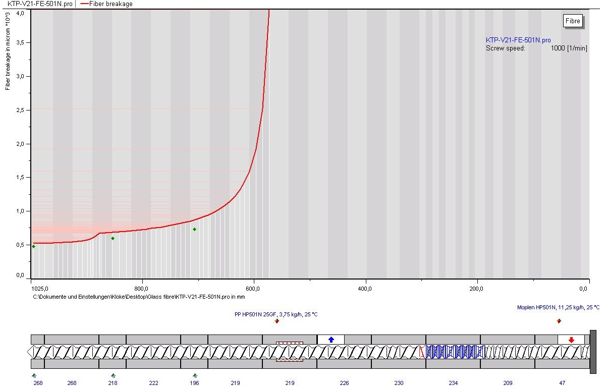
Figure 7: Glass fiber length reduction along the screw length of an operating point
In the figure the glass fiber length is depicted from the feeding point to the screw tip. The y-axis shows for each interval the calculated glass fiber length in µm. The bend in the course of the function results from the changed flow conditions because of the filled sections caused by the back flow length.
The glass fiber length in the compound thus determined has been calculated for all further operating points. Figure 8 and Figure 9 show a comparison of the measured glass fiber length above the calculated ones.
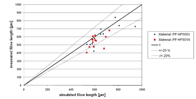
Figure 8: Measured above calculated fiber length; mixing zone: kneading block 90° staggering angle
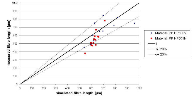
Figure 9: Measured above calculated fiber length; mixing zone: Conveying elements 36/36
Carbon fiber fracture modeling
The following equation is used as a basis for the fiber degradation progress as a function:
$$\frac{dl}{dt} = -k \cdot l \tag{22}$$
To calculate the fiber length reduction over time, the fiber breakage rate k and the fiber length l must be known. The rate includes all mechanical processes that can lead to breakage. The bending load can be calculated using the bending moment M, the axial moment of inertia I and the maximum center distance amax. By inserting the moment of inertia I and the fiber radius d /2 for amax and by reformulating the bending moment, the equation changes as follows [Sko18]:
$$\sigma_{Randfaser} = \frac{M}{I} \cdot a_{max} = = \frac{F_{Strömung} \cdot y_{max}}{\frac{\pi \cdot d^4}{64}} \cdot \frac{d}{2} \tag{23}$$
The equivalent force Fflow is determined from the shear stress of the flow σflow and the sheath area of a fiber Asheath [Sko18].
Mit $\sigma_{Strömung} = \eta \cdot \dot{\gamma}_{Strömung}$ und $A_{Mantel} = \pi \cdot d \cdot l$ ergibt sich:
$$F_{Strömung} = \pi \cdot d \cdot l \cdot \eta \cdot \dot{\gamma}_{Strömung} \tag{24}$$
The maximum deflection of the fiber is described by the following equation [TG61]:
$$y_{max} = \frac{\sqrt{8}}{\pi} \cdot \sqrt{1 - \frac{F_{Euler}}{F_{Strömung}}} \cdot l \tag{25}$$
In addition to the force from the flow, the force that a fiber can withstand, $F_{Euler}$ is calculated based on Euler buckling theory [CM72].
$$F_{Euler} = \frac{\pi^3 \cdot d^4}{64 \cdot l^2} \cdot E \tag{26}$$
In order for a fiber to buckle, the force generated by the flow must be at least equal to or greater than the force that a fiber can withstand. Therefore, the breaking criterion can be summarized as follows:
$$\frac{\sigma_{Randfaser}}{\sigma_{Bruch}} = \frac{F_{Strömung} \cdot y_{max}}{l} \cdot \frac{a_{max}}{\varepsilon \cdot E_{CF}} \tag{27}$$
If this is taken as the breakage criterion $k$, the fiber breakage is based on the following equation:
$$\frac{dl}{dt} = -\frac{F_{Strömung} \cdot y_{max}}{l} \cdot \frac{a_{max}}{\varepsilon \cdot E_{CF}} \cdot l \cdot \frac{1}{t} \tag{28}$$
With all the values used for the input variables of the fiber ($d,ε,E_CF,l$) and output variables of an extruder simulation ($η,γ̇,t$) the following is obtained:
$$k(t,l) = -\frac{32 \cdot \eta \cdot \dot{\gamma} \cdot l^2 \cdot \sqrt{8}}{d^2 \cdot \varepsilon \cdot E_{CF} \cdot \pi} \cdot \sqrt{1 - \frac{\pi^2 \cdot E_{CF} \cdot d^3}{64 \cdot \eta \cdot \dot{\gamma} \cdot l^3}} \cdot \frac{1}{t_r} \tag{29}$$
To enable an analytical solution, the differential equation is transformed into individual differences [HMR+21]:
$$\frac{l_i - l_{i-1}}{\Delta t} = -\frac{32 \cdot \eta \cdot \dot{\gamma} \cdot l_{i-1} \cdot \sqrt{8}}{d^2 \cdot \varepsilon \cdot E_{CF} \cdot \pi} \cdot \sqrt{1 - \frac{\pi^2 \cdot E_{CF} \cdot d^3}{64 \cdot \eta \cdot \dot{\gamma} \cdot l_{i-1}^3}} \cdot \frac{1}{t} \cdot l_{i-1}^2 \tag{30}$$
Nomenclature
| Symbol | German | English |
|---|---|---|
| $\sigma_{Bruch}$ | Faserbruchspannung | Fiber fracture stress |
| $\sigma_{Randfaser}$ | Randfaserspannung | Edge fiber stress |
| $F_{Strömung}$ | Kraft aus der Strömung | Force from the flow |
| $E_{CF}$ | Elastizitätsmodul | Young's modulus |
| $a_{max}$ | maximalen Achsabstandes | maximum center distance |
| $y_{max}$ | Maximale Faserdurchbiegung | Maximum fiber deflection |
| $I$ | Axiales Trägheitsmoment | Axial moment of inertia |
| $\varepsilon$ | Bruchdehnung | Elongation at break |
| $T$ | Verweilzeit | Residence time |
References
[Ans93] J. Ansahl: „Grundlagen für die Auslegung dichtkämmender Gleichdrall Doppelschneckenextruder“, Dissertation, Universität Paderborn, 1993
[BG97] W. Beitz, K.-H. Grote, „DUBBEL Taschenbuch für den Maschinenbau“, 19. Auflage, Springer Verlag, München, 1997
[CM72] CHMELKA, F. und E. MELAN, 1972. Einführung in die Festigkeitslehre für Studierende des Bauwesens. Fünfte, verbesserte und ergänzte Auflage. Vienna: Springer Vienna. ISBN 978-3-7091-8305-2
[HMR+21] Helmlinger, L., Malatyali, H., Rudloff, J., Lang, M., Schöppner, V., Hochrein, T., Bastian, M., 2021. Untersuchung des Compoundierprozesses von Carbonfaserrezyklaten. SKZ - Das Kunststoff-Zentrum (Hrsg.), ISBN: 978-3-8440-7946-3, Shaker-Verlag
[Mel98] U. Melisch: „Grundlagen zur Simulation des Förder- und Plastifizierprozesses dichtkämmender Gleichdrall-Doppelschneckenextruder“, Dissertation, Universität Paderborn, 1998
[Sko18] SKOLAUT, W., Hg., 2018. Maschinenbau. Ein Lehrbuch für das ganze Bachelor-Studium [online]. 2., aktualisierte und überarbeitete. Berlin: Springer Vieweg. ISBN 9783662558812
[TG61] TIMOŠENKO, S.P. und J.M. GERE, 2000. Theory of elastic stability. 2. ed., [Nachdr.], internat. student ed. Auckland: McGraw-Hill. Engineering societies monographs. ISBN 9780070858213