The energy equation for the calculation of the radial temperature profile in the screw flight forms the basis for the 2D model.

$$\rho c \left(\frac{\partial T}{\partial t} + v \nabla T\right) = \lambda \nabla^2 T + \tau \nabla v \tag{Equation 1}$$

A modification of the energy equation to match the existing open system, which exchanges the energy and the mass with the environment, follows.

The cylinder moves as an ideally formed plate over the rigid screw, so that one can resort back to a pan model with kinematic reversal. The different diction for Cartesian coordinates results in the following function for the energy equation with the aforementioned geometry. [Sch13]

$$\rho c \left(\frac{\partial T}{\partial t} + v_x \frac{\partial T}{\partial x} + v_y \frac{\partial T}{\partial y} + v_z \frac{\partial T}{\partial z}\right) = -\left(\frac{\partial \dot{q}_x}{\partial x} + \frac{\partial \dot{q}_y}{\partial y} + \frac{\partial \dot{q}_z}{\partial z}\right)$$

$$-T \left(\frac{\partial p}{\partial T}\right)_V \left(\frac{\partial v_x}{\partial x} + \frac{\partial v_y}{\partial y} + \frac{\partial v_z}{\partial z}\right) - \left(\sigma_{xx} \frac{\partial v_x}{\partial x} + \sigma_{yy} \frac{\partial v_y}{\partial y} + \sigma_{zz} \frac{\partial v_z}{\partial z}\right) $$

$$-\left[\tau_{xy} \left(\frac{\partial v_y}{\partial x} + \frac{\partial v_x}{\partial y}\right) + \tau_{xz} \left(\frac{\partial v_z}{\partial x} + \frac{\partial v_x}{\partial z}\right) + \tau_{yz} \left(\frac{\partial v_y}{\partial z} + \frac{\partial v_z}{\partial y}\right)\right]\tag{Equation 2}$$

The equation consists of five terms, which have the following meanings [Ang10]:

• The left side equates to the change of the internal energy per unit of time and volume
• The first term on the right equates to the change of the supplied energy through heat conduction per unit of time and volume
• The second term on the right equates to the recoverable amount of work per unit of time and volume through compression
• The third and fourth terms on the right side equate to the non-recoverable amount of work per unit of volume and time as a result of dissipation

As to obtain an analytic result, the equation must be simplified with further model assumptions. Apart from the viscosity, all material parameters are presumed temperature independent.

In addition to the aforementioned ones, further assumptions are also made [Sch13]:

• The flow is stationary and laminarily following ($\frac{\partial T}{\partial t} = 0$)
• As the polymer melt is seen as incompressible ($\rho = konst.$), the second term disappears on the right side of the energy equation. Therefore the examination of the thermal capacity becomes simpler ($c_p = c_v = c$)
• In the direction of x and y no speed components are examined ($v_x = v_y = 0$)
• The screw canal is completely filled with the melt, which is wall-adhering
• The heat flows in the direction of the flight and those transverse to them can be neglected in comparison to the heat flow in the direction of the flight height ($q_x = q_z = 0$)
• Because the flight height is considerably smaller than the flight width ($h << b$), the shear stresses at the supporting flights can be neglected ($\tau_{xz} = 0$)
• Normal stresses are also neglectable ($\sigma_{xx} = \sigma_{yy} = \sigma_{zz} = 0$)

With the help of the simplifying criteria the equation 4-2 can be reduced to 3 terms:

$$\rho c v_z \frac{\partial T}{\partial z} = -\frac{\partial \dot{q}_y}{\partial y} - \tau_{yz} \left(\frac{\partial v_z}{\partial y}\right)\tag{Equation 3}$$

The sum of thermal conduction in the flight height and the energy of the dissipation results in the temperature rising lengthways in the canal, which is filled with polymer melt.

Under consideration of the Fourier thermal conductivity approach for the heat flow in direction of the flight height and the power flow law for non-newtonian flow behavior of polymer melt with the Arrehnius-approach, the equation 4-3 can be extended to the following:

$$\rho c \bar{v}_z \frac{\partial T}{\partial z} = \lambda \frac{\partial^2 T}{\partial y^2} + \left(\overline{\tau\dot{\gamma}}\right)_0 e^{-\beta(T-T_0)}\tag{Equation 4}$$

To simplify the energy equation further, the dimensionless operating figures as described in [Ang10], the Graetz- ($Gz$) and the Brinkmann-number ($Br$), are used. Herein, the Brinkmann-number describes the relation of disperse energy in the screw canal to the heat conduction in the direction of the flight height. The Graetz-number describes the convection in the direction of the flight length to the heat conduction in the direction of the flight height. Additionally, the dimensionless coordinates $\xi$, $\zeta$ and the dimensionless temperature $\Theta$ are placed in the energy equation.

$$Br = \frac{\left(\overline{\tau\dot{\gamma}}\right)_0 h^2}{\lambda T_Z} \approx \frac{K_{0T} v_0^{1+n} h^{1-n}}{\lambda T_Z}\tag{Equation 5}$$

$$Gz = \frac{c \rho \bar{v}_z h^2}{\lambda \Delta z} = \frac{c \rho h}{\lambda b \Delta z} \dot{V}\tag{Equation 6}$$

$$\Theta = \frac{T - T_0}{T_Z}\tag{Equation 7}$$

$$\xi = \frac{\Delta y}{h}\tag{Equation 8}$$

$$\zeta = \frac{\Delta z}{l}\tag{Equation 9}$$

During the geometric calculation of the Graetz- $Gr$ and Brinkmann-number $Br$ some twin screw-specific adjustments are made. For the ascertainment of the Graetz-number $Gr$ the flight height $h$ and the flight width $br$ are important. These two sizes are defined using the average flight height $\bar{h}$ and the flight width $b_{max}$ of the twin screw extruder.

For the Brinkmann-number $Br$ the viscosity $\eta$ is needed, this depends on the shear rate $\dot{\gamma}$ and is influenced by the geometry of the twin screw extruder. As there is no constant flight height $h$ in the canal, the average flight height $\bar{h}$ is used to calculate the average shear rate $\overline{\dot{\gamma}}$. Without considering the influence of the characteristics of the screw element (mixing elements, Shear elements etc.), [Kre04]

$$\overline{\dot{\gamma}} = \frac{\bar{h}}{v_0}\tag{Equation 10}$$

The function for the calculation of the temperature in the melt-filled canal, assumes the following shape:

$$\frac{\partial \Theta}{\partial \xi} = \frac{1}{Gz} \frac{\partial^2 \Theta}{\partial \xi^2} + \frac{Br}{Gz} \exp\left[-\beta(T_Z \Theta)\right]\tag{Equation 11}$$

It is not possible yet, to solve the, as the exponential term is dependent on the temperature $T$ or rather $\Theta$. In the following equation the exponential term is partly linearized.

$$\exp\left[-\beta(T - T_0)\right] = \exp\left[-\beta(T_Z \Theta)\right] = c_1 - c_2 \beta T_Z \Theta\tag{Equation 12}$$

This linear equation divides the exponential term into two parts. The first part is dependent on the radial temperature $T$ or rather $\Theta$ ($c_2 \beta T_Z \Theta$) and the second is dependent on $T$ or rather $\Theta$ and $c_1$. The two unknown parameters $c_1$ and $c_2$ are calculated in two equations, which approach the exponential function with a secant which lies between the average radial temperature of the previous section $T_0$ and the cylinder wall temperature $T_Z$.

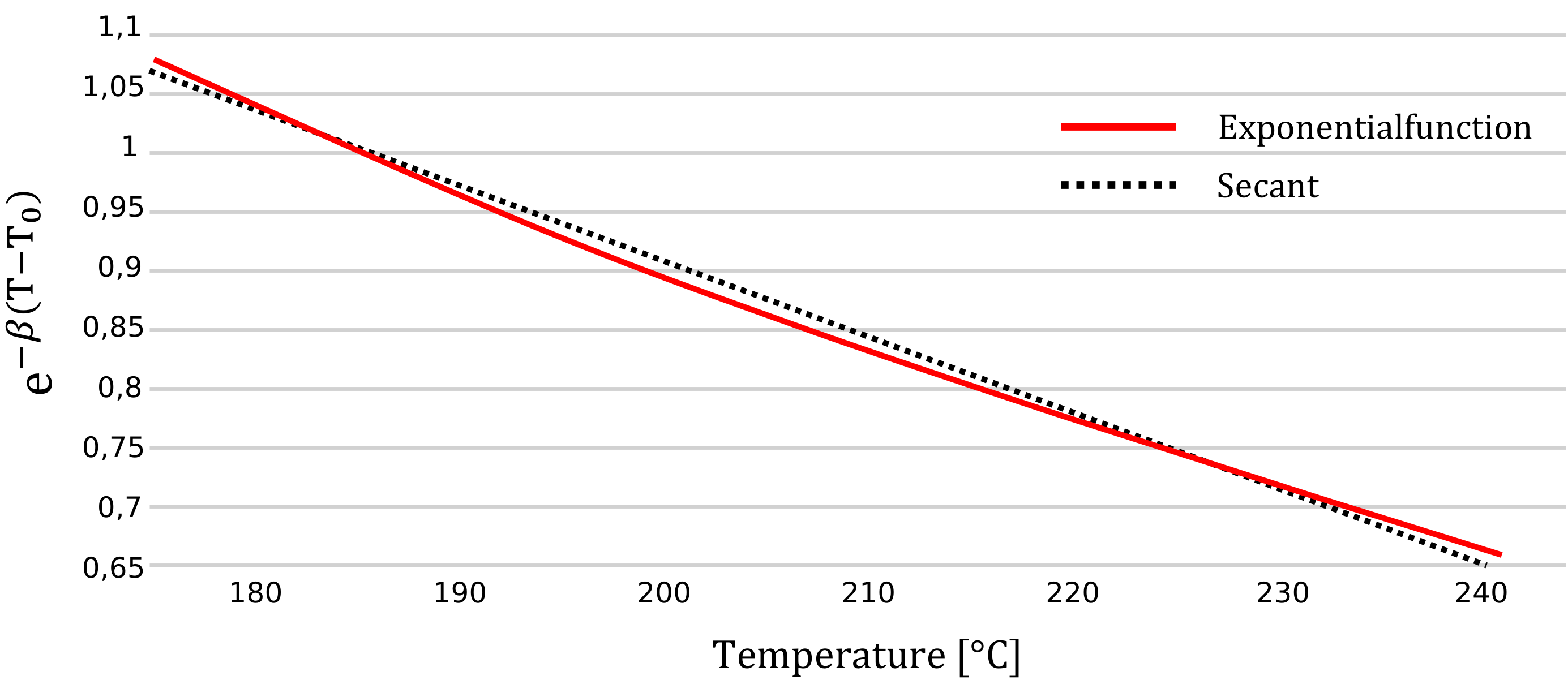
Image 1: approach of exponential function using a secant [Ang10]

In summary, the linearization with the Equation 10 produces the analytically solvable, simplified energy equation for the radial temperature (for $0 \leq \xi \leq 1$ and $0 \leq \zeta \leq 1$) [Ang10]:

$$\frac{\partial^2 \Theta}{\partial \xi^2} - Gz \frac{\partial \Theta}{\partial \xi} - c_2 \beta T_Z Br \Theta = -c_1 Br\tag{Equation 13}$$

The presented differential equation was successfully solved with the marginal conditions of the constant cylinder temperature and a tempered screw in the elaboration of [Sch13]. This model was adjusted according to the calculation of the temperature progression in the co-rotating twin screw extruder. As the solution contains dimensionless temperature data, these must still be converted into dimensioned data.

This can be done using the following equation and results in the ten data of the profile of the flight height.

$$T_{0,n}(\xi) = \theta_{\xi,n} T_{Z,n} + T_{n-1}\tag{Equation 14}$$

Finally the arithmetic mean is formed from the radial temperature data and the average canal temperature of the section is defined. Because of the step-by-step calculation in SIGMA the axial temperature curve can be calculated.