Dies ist eine alte Version des Dokuments!
Melt Temperature
Original Model
The temperature is based on channel the model. The following prerequisites need to be carried out:
- The screw channel is to be considered shallow i.e. $b >> h$. The influence of the flights can be neglected.
- The melt is wall sticking.
- The flow is laminar, creeping and incompressible ($c=c_v =c_p$).
- The behavior of the flow of the melt should follow that of the power law $\tau = K \cdot \dot{\gamma}^n$.
- For all of the physical properties, average values are used (with the exception of the viscosity).
- The material flow is considered through the introduction of the average effective channel widths and channel height.
The describing differential equation results with these simplifying assumptions for a constant zone geometry [Pot91].
$$\rho c \bar{V}_z \frac{\partial T}{\partial z} = \lambda \frac{\partial^2 T}{\partial y^2} + \overline{(\tau\dot{\gamma})}_0 e^{-\beta(T-T_0)} \tag{1}$$
The left side describes the temperature increase in the channel direction z, the first term of the right side considers the thermal conductivity in the channel height direction y. The second term describes the dissipated energy $(\overline{\tau \gamma})_0$ over the channel cross section averaged dissipated power consumption, per unit volume at a temperature of $T_0$.
Dimensionless characteristics for the temperature estimation
$$\Theta_0 = \frac{T_0 - T_z}{T_Z} \qquad \xi = \frac{y}{h} \qquad \zeta = \frac{z}{Z}$$
$$Br = \frac{(\tau \gamma)_0 \overline{h}^2}{\lambda T_Z} \approx \frac{K v_0^{1+n} \overline{h}^{1-n}}{\lambda T_Z}$$
$$Gz = \frac{c_p \rho \overline{h} V}{\lambda \overline{b} Z k}$$ With the introduction of the dimensionless characteristics described in table follows:
$$Gz \frac{\partial \Theta}{\partial \zeta} = \frac{\partial^2 \Theta}{\partial \xi^2} + Br \cdot e^{-\beta T_z \Theta} \tag{2}$$
Due to the exponential function, the differential equation can no longer be solved. In [Pot91], [Koc87], [Sch90] the exponential function was represented through a set of linear equations of the form:
$$e^{-\beta(T-T_0)} = c_1 - c_2 \beta (T - T_0) \tag{3}$$
This will be shown in the figure.
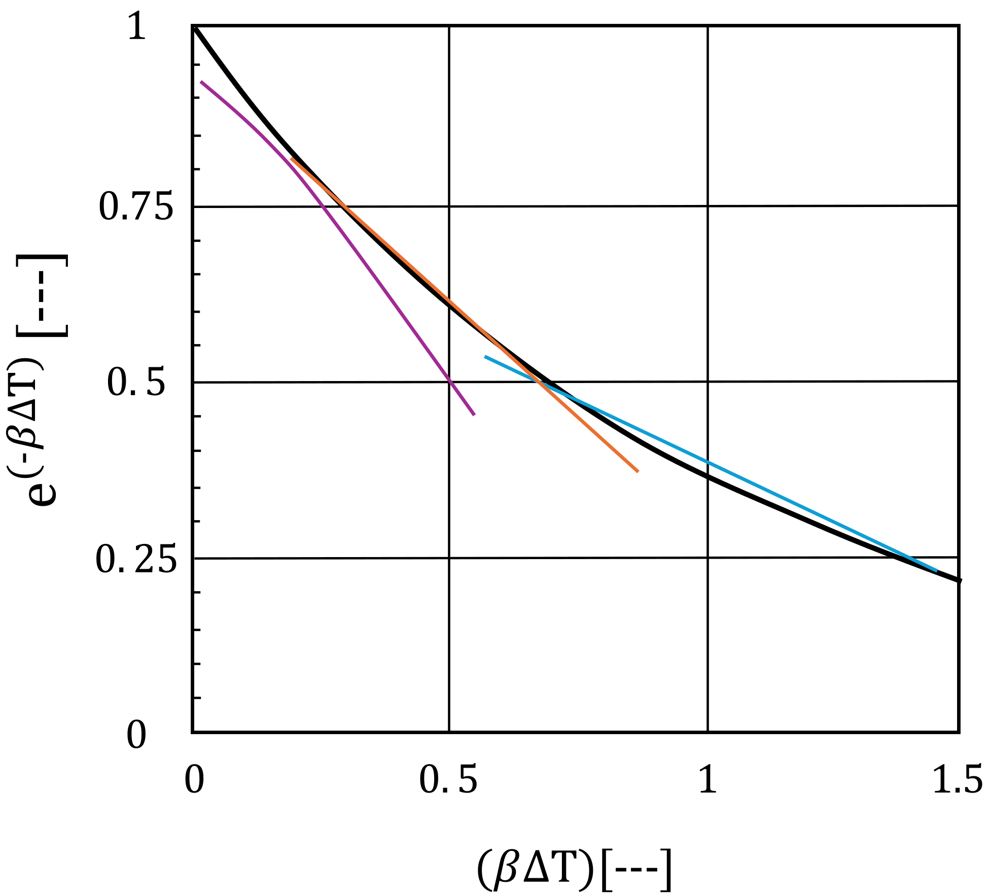
Figure: Approximation of the exponential function through a set of linear equations [Pot91], [Koc87], [Sch90]
If one assumes the estimation to be performed in small sections then the simplifications are possible. In small sections it can be assumed that the difference in the temperature in the channel direction is small and therefore the equation (4) follows:
$$\beta \Delta T \to 0 \tag{4}$$
From this equation (5) results:
$$\frac{\partial^2 \Theta}{\partial \xi^2} - Gz \frac{\partial \Theta}{\partial \xi} = -Br \tag{5}$$
This differential equation was solved in [SA90], [CJ59]. If the heat source is independent from the coordinate z, the following prerequisites are used:
Prerequisites
- For the area $x > 0$ the rule for the starting temperature profile $\Theta(z=0)=\Theta_0=\Theta_{Start}+m*x$ respectively the average start temperature $\Theta(z=0)=\Theta_{Start}$ for $m = 0$
- The heat source per coordinate unit $\Delta z$ and volume unit for $z > 0$ as average has to be included in the estimation.
- The barrel temperature $T_Z$ is constant.
On approaching the screw, the temperature reaches a limiting value (semi infinite space). Using small sections and taking into account the actual geometry of the channel, the limiting value is almost achieved. Hence the boundary condition that is used is comparable to the one of an adiabatic screw where the limiting value is always reached exactly.
With the above mentioned boundary and initial conditions we reach the solution shown in table [4, 5].
Solution for the temperature estimation
$$\Theta(\zeta, \xi) = \left[\Theta_0 + \frac{Br}{Gz} \zeta + \frac{Br}{Gz} \xi^2\right] \text{erf}\left(\frac{\xi}{2\sqrt{\frac{\zeta}{Gz}}}\right) + Br \xi \sqrt{\frac{\zeta}{Gz}} e^{[-\frac{Gz\xi^2}{4\zeta}]} - \frac{Br}{2} \xi^2$$
$$\bar{\Theta} = \frac{\bar{T} - T_Z}{T_Z} = \int_0^1 \Theta(\zeta, \xi) d\xi$$
In every heating zone a constant wall temperature is imposed. The temperature calculation starts at the point where the first melt is found. This is the place of the first melt pool formation, at the start of the melting respectively.
The average start temperature $\bar{\Theta}_{Start}$ is calculated using the energy equation for the melt layer on the barrel wall. The energy equation for the melt layer on the barrel wall is [Pot91], [Sch90]:
$$\lambda_s \frac{\partial^2 T}{\partial y^2} + \tau_{yi} \frac{\partial v_j}{\partial y} = 0 \tag{6}$$
With the boundary conditions $T(0) = T_{Fl}$ und $T(\delta) = T_Z$ one reaches the following solution:
$$T(\xi) = T_{Fl} + (T_Z - T_{Fl}) \left\{\xi + Br \left[\frac{1}{A^2}\left(\frac{A}{e^A - 1}\right)^{1+n}\left(1 - e^{A\xi} - \xi(1 - e^A)\right)\right]\right\} \tag{7}$$
with:
$$Br = \frac{K(T_{Fl})v_{rel}^{1+n} \overline{\delta}^{1-n}}{\lambda_s (T_Z - T_{Fl})} \tag{8}$$
and
$$\xi = \frac{y}{\delta} \tag{9}$$
$$A = \frac{\beta(T_Z - T_{Fl})}{n} \tag{10}$$
From it we get the average temperature for the melt layer under the consideration of the velocity profile:
$$\bar{T} = T_{Start} = \frac{\int_0^1 v(\xi)T(\xi)d\xi}{\int_0^1 v(\xi)d\xi} \tag{11}$$
and
$$v(\xi) = v_{rel} \frac{e^{A\xi} - 1}{e^A - 1} \tag{12}$$
Equations to estimate the average starting temperature
$$T_{Start} = [B \Delta T(A - 1)2e^{2A} - (AB \Delta T e^{2A} + A_3 - A2)]A_4$$
$$B = Br \frac{1}{A^2} \left[\frac{A}{e^A - 1}\right]^{1+n} \qquad \Delta T = T_Z - T_{Fl} A = \frac{\beta}{n} \Delta T$$
$$A_1 = A^2(B + 1) + 3AB + 2(B - 1)$$
$$A_2 = [\Delta T(A(B + 1) + 2B - 1) + AT_{Fl}]2e^A$$
$$A_3 = A^2B \Delta T e^A + \Delta T A_1 + 2AT_{Fl}(A + 1)$$
$$A_4 = \frac{1}{2A(e^A - A - 1)}$$
As Solution one obtains the equations, which are listed in the table. The average temperature for the melt layer is the same as that of the average temperature for the temperature flow estimation. Under the assumption $Br = 0$ the average starting temperature can be solved with the simple solution [1, 6]:
$$\bar{T}_{\mathrm{start}} = T_{\mathrm{Fl}} + (T_Z - T_{\mathrm{Fl}}) \cdot \frac{\frac{1}{A} - 1 + e^A \left(1 - \frac{1}{A}\right)}{e^A - A - 1}$$
Modified Model
In the figure the results of a couple of models for the estimation of the temperature development are confronted with the results of non-isothermal flow simulations.
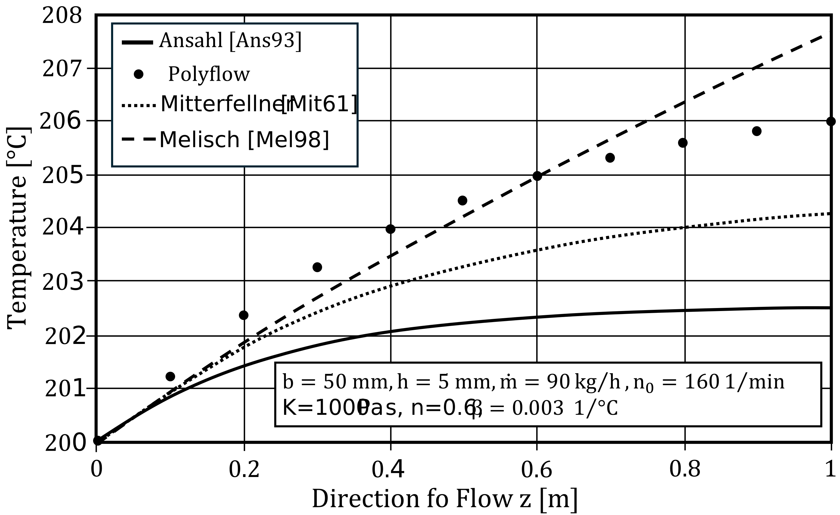
Figure: Comparison of existing models for the estimation of the melt temperature.
In the approaches of Ansahl [8] und Melisch [7] the temperature development is underestimated. In the approach of Mitterfellner [9], however, it is overestimated. What is more, it attracts the attention that with an increasing channel length the trend, i.e. the approximation to a limiting temperature, is not represented in a correct way in the model of Mitterfellner.
The general energy equation is the starting basis for the estimation of the temperature:
$$\rho \cdot c \left( \frac{\partial T}{\partial t} + v_x \frac{\partial T}{\partial x} + v_y \frac{\partial T}{\partial y} + v_z \frac{\partial T}{\partial z} \right) = \left( \frac{\partial \dot{q}_x}{\partial x} + \frac{\partial \dot{q}_y}{\partial y} + \frac{\partial \dot{q}_z}{\partial z} \right) $$ $$- T \left( \frac{\partial p}{\partial T} \right)_{\rho} \left( \frac{\partial v_x}{\partial x} + \frac{\partial v_y}{\partial y} + \frac{\partial v_z}{\partial z} \right) - \left[ \tau_{xx} \frac{\partial v_x}{\partial x} + \tau_{yy} \frac{\partial v_y}{\partial x} + \tau_{zz} \frac{\partial v_z}{\partial x} \right] $$ $$- \left[ \tau_{xy} \left( \frac{\partial v_x}{\partial y} + \frac{\partial v_y}{\partial x} \right) + \tau_{zx} \left( \frac{\partial v_x}{\partial z} + \frac{\partial v_z}{\partial x} \right) + \tau_{zy} \left( \frac{\partial v_y}{\partial z} + \frac{\partial v_z}{\partial y} \right) \right] \tag{1}$$
To receive a mathematically clear and closed solution, the following simplifying assumptions are made:
- The melt is wall-adherent.
- The flow be stationary, incompressible and laminar creeping ($c = c_v = c_p$).
- The flow properties of the melt comply with the power law: $\tau = K \cdot \dot{\gamma}^n$.
- All material values, except the viscosity, are considered as being temperature invariant. For polymer melts this assumption is a feasible approximation as long as the temperature range is not too large.
- The dissipated energy is calculated by means of the approach introduced in chapter Estimation of the Power Consumption and is standardized to a reference temperature of $T_\infty$.
- For the temperature dependence of the flow law coefficient $K(T)$ the simplified Arrhenius approach seems to be appropriate: $K(T) = K(T_0) \cdot e^{-\beta(T-T_0)}$
- The coordinate system is lying on the screw root surface (see figure).
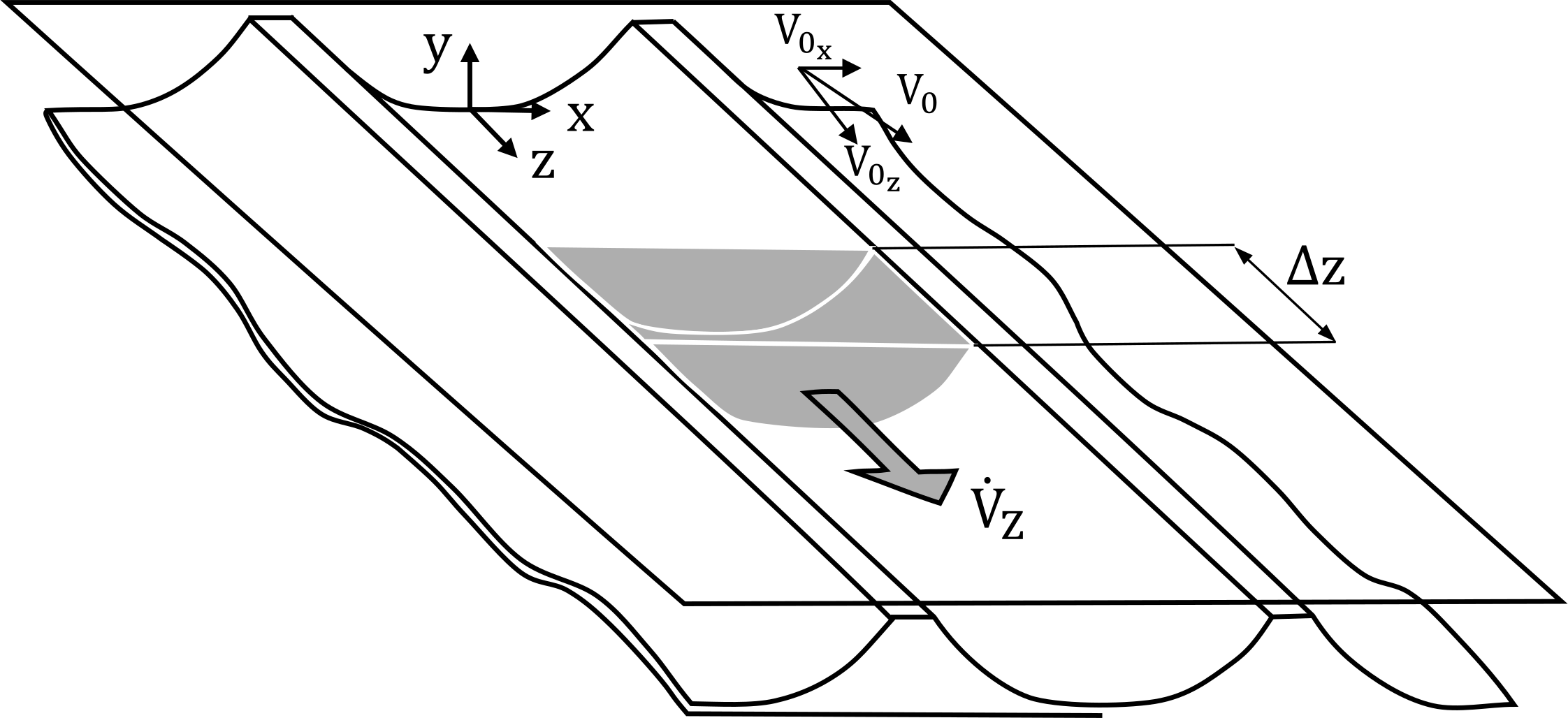 Figure: Conveyor channel model for the estimation of the temperature development in the channel.
Under these assumptions the energy equation simplifies to:
$$\frac{\partial T}{\partial z} = -\frac{1}{\rho \cdot c \cdot \bar{v}_{0z}} \cdot \frac{\partial \dot{q}_y}{\partial y} + \frac{\overline{ ({\tau} \cdot {\gamma})_j }}{\rho \cdot c \cdot \bar{v}_{0z}} \cdot e^{-\beta (T - T_j)} \tag{2}$$
For the heat flow the Fourier's law for heat conduction may apply
$$\dot{q}_y = -\lambda \frac{\partial T}{\partial y} \tag{3}$$
Is the differential equation standardized, then follows in conjunction with the dimensionless parameters defined in the table:
$$\frac{\partial \Theta}{\partial \zeta} = \frac{1}{Gz} \cdot \frac{\partial^2 \Theta}{\partial \xi^2} + \frac{Br}{Gz} e^{-\beta T_z \Theta} \tag{4}$$
Table: Dimensionless factors for the temperature estimation.
| Parameter | Definition |
|---|---|
| $ \Theta_{0} $ | $ \frac{T_{0} - T_{j}}{T_{z}} $ |
| $ \Theta $ | $ \frac{T - T_{j}}{T_{z}} $ |
| $ \xi $ | $ \frac{y}{\bar{h}} $ |
| $ \zeta $ | $ \frac{z}{\Delta z} $ |
| $ Br $ | $ \frac{ \left( \overline{ \tau \cdot \dot{\gamma} } \right)_j \bar{h}^2 }{ \lambda T_z } $ |
| $ Gz $ | $ \frac{ c \cdot \rho \cdot \bar{h} \cdot \dot{V}_{z} }{ \lambda \bar{b} \Delta z } $ |
Due to the exponential term the partial differential equation (4) cannot be solved analytically. In accordance to Melisch [7] this term is linearized. The following equation results:
$$\frac{\partial \Theta}{\partial \zeta} = \frac{1}{Gz} \cdot \frac{\partial^2 \Theta}{\partial \xi^2} + \frac{Br}{Gz} \cdot (C_1 - C_2 \cdot \beta \cdot T_z \cdot \Theta) \tag{5}$$
The factors $C_1$ and $C_2$ are defined in [7]. The solution of this differential equation describes the temperature change for a zone with constant geometry as well as invariant material properties (except the influence of the viscosity). To comply with these requirements the estimation has to be performed in small sections.
The Channel Area
For the resolution of the equation (1) the starting temperature $T_0$ of the mathematical interval is selected as reference temperature. The coordinate system is laid on the screw root surface.
For the resolution of the differential equation it is assumed that the temperature differences in an interval $\Delta z$ are diminutive. The temperature equalization processes, which are to be expected in direction of the screw channel depth, are therefore approximately constant and almost independent of the z-coordinate for a certain calculation section.
$$\frac{\partial^2 \Theta}{\partial \xi^2} \approx \frac{\partial^2 \Theta_0}{\partial \xi^2} \tag{1}$$
Consequently, the alteration of the heat flow in $\xi$-direction can be estimated in a simplifying way on the basis of the starting temperature profile. A potential equation for the specification of the temperature profile in direction of the screw channel depth is Equation (2).
$$\Theta_0 = \Theta_z + (K_1 + K_2) \cdot \xi^2 + K_1 \cdot \xi^4 + K_2 \cdot \xi^6 \tag{2}$$
The following boundary conditions were applied for the resolution of the differential equation:
- Heat transfer to the screw does not take place: $\frac{\partial \Theta}{\partial \xi} = 0$ für $\xi = 0 \tag{3}$
- A predetermined temperature $T_{z}$ is found at the barrel wall:
$$\Theta(\zeta, \xi = 1) = \Theta_z = \frac{T_z - T_0}{T_z} \tag{4}$$
- The medium melt temperature is known at the beginning of the calculation section:
$$\int_0^1 \Theta(\zeta = 0, \xi) \cdot d \xi = \frac{T_0 - T_0}{T_z} = 0 \tag{5}$$
From this the following solution of equation (1) derives:
$$\Theta(\zeta, \xi) = \frac{2 \cdot K_1 - 2 \cdot K_2 + 12 \cdot K_1 \cdot \xi^2 + 30 \cdot K_2 \cdot \xi^4 + Br \cdot C_1}{Br \cdot C_2 \cdot \beta \cdot T_z} \cdot (1 - \varepsilon)$$
$$+ (\Theta_z + (K_1 - K_2) \cdot \xi^2 +) \cdot K_1 \cdot \xi^4 + K_2 \cdot \xi^6) \cdot \varepsilon \tag{6}$$
with
$$K_1 = -\frac{5}{2} \cdot \frac{147 \cdot (\Theta_z - \varepsilon) + Br \cdot C_2 \cdot (1 - \varepsilon) + Br \cdot C_2 \cdot \beta \cdot T_z \cdot \Theta_z \cdot (\varepsilon - 1)}{231 \cdot (1 - \varepsilon) + 5 \cdot \varepsilon \cdot Br \cdot C_2 \cdot \beta \cdot T_z \cdot \Theta_z} \tag{7}$$
$$K_2 = \frac{7}{4} \cdot \frac{105 \cdot \Theta_z \cdot (1 - \varepsilon) + 4 \cdot Br \cdot C_2 \cdot (\varepsilon - 1) + Br \cdot Gz \cdot \beta \cdot T_z \cdot \Theta_z \cdot (4 + 11 \cdot \varepsilon)}{231 \cdot (1 - \varepsilon) + 5 \cdot \varepsilon \cdot Br \cdot C_2 \cdot \beta \cdot T_z \cdot \Theta_z} \tag{8}$$
The medium temperature in the channel is calculated with:
$$\varepsilon = e^{\left(-\frac{Br \cdot C_2 \cdot \beta \cdot T_z}{Gz} \zeta\right)} \tag{9}$$
$$\overline{\Theta} = \frac{\overline{T} - T_0}{T_z} = \int_0^1 \Theta(\xi, \zeta) \cdot d \xi \tag{10}$$
This results in:
$$\overline{\Theta} = \frac{K_2 \cdot \varepsilon}{7} + \frac{C_1 \cdot (1 - \varepsilon)}{C_2 \cdot \beta \cdot T_z} + \Theta_z \cdot \varepsilon + K_1 \cdot \frac{6 - 6 \cdot \varepsilon + \frac{8}{15} \cdot \varepsilon \cdot Br \cdot C_2 \cdot \beta \cdot T_z}{Br \cdot C_2 \cdot \beta \cdot T_z}$$
$$+K_2 \cdot \frac{4 - 4 \cdot \varepsilon - \frac{1}{3} \cdot \varepsilon \cdot Br \cdot C_2 \cdot \beta \cdot T_z}{Br \cdot C_2 \cdot \beta \cdot T_z} \tag{11}$$
For a first verification the model predictions were confronted with the results of non-isothermal flow simulations. The figure exhibits the comparison of the medium temperatures. An improvement of the description quality can be observed here as compared to the models published so far.
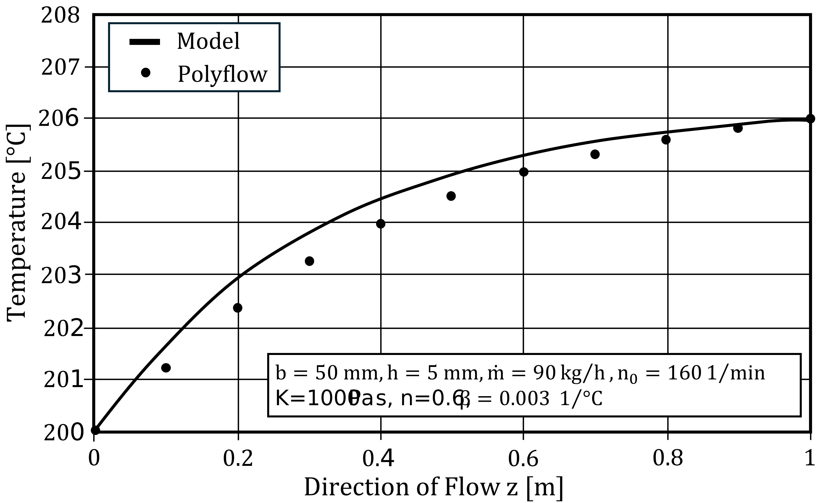
Figure: Comparison of the model predictions with the polyflow results for rectangular channels.
The figure displays a further comparison of the calculated medium temperatures for a twin screw channel. Here also a good accordance could be observed between the simulation results and the model predictions.
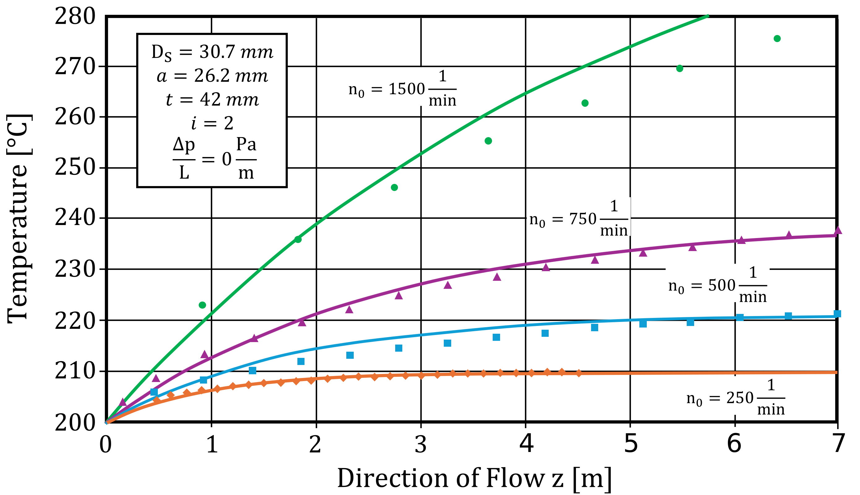
Figure: Comparison of the model with Polyflow results for twin screw channels.
Radial Clearance and Groove Flow
The temperature increase in the radial clearance and in the grooves can be calculated with the same approach as the one, with which the temperature increase is determined in the channel.
$$\frac{\partial T}{\partial x} = -\frac{1}{\rho \cdot c \cdot \overline{v}_{0x}} \cdot \frac{\partial \dot q}{\partial y} + \frac{\overline{(\tau \cdot \dot{\gamma})}_j}{\rho \cdot c \cdot \overline{v}_{0x}} \cdot e^{-\beta(T-T_i)} \tag{1}$$
Is the differential equation standardized, then follows in conjunction with the dimensionless parameters defined in the table:
$$\frac{\partial \Theta}{\partial \zeta} = \frac{1}{Gz} \cdot \frac{\partial^2 \Theta}{\partial \xi^2} + \frac{Br}{Gz} e^{-\beta \cdot T_z \cdot \Theta} \tag{2}$$
The resolution of the differential equation is performed analogous to chapter The Channel Area. One receives:
$$\overline{\Theta} = \frac{K_2 \cdot \varepsilon}{7} + \frac{C_1 \cdot (1 - \varepsilon)}{C_2 \cdot \beta \cdot T_z} + \Theta_z \cdot \varepsilon + K_1 \cdot \frac{6 - 6 \cdot \varepsilon + \frac{8}{15} \cdot \varepsilon \cdot Br \cdot C_2 \cdot \beta \cdot T_z}{Br \cdot C_2 \cdot \beta \cdot T_z}$$
$$+K_2 \cdot \frac{4 - 4 \cdot \varepsilon - \frac{1}{3} \cdot \varepsilon \cdot Br \cdot C_2 \cdot \beta \cdot T_z}{Br \cdot C_2 \cdot \beta \cdot T_z} \tag{3}$$
with:
$$K_1 = -\frac{5}{2} \cdot \frac{147 \cdot (\Theta_z - \varepsilon) + Br \cdot C_2 \cdot (1 - \varepsilon) + Br \cdot C_2 \cdot \beta \cdot T_z \cdot \Theta_z \cdot (\varepsilon - 1)}{231 \cdot (1 - \varepsilon) + 5 \cdot \varepsilon \cdot Br \cdot C_2 \cdot \beta \cdot T_z \cdot \Theta_z} \tag{4}$$
$$K_2 = \frac{7}{4} \cdot \frac{105 \cdot \Theta_z \cdot (1 - \varepsilon) + 4 \cdot Br \cdot C_2 \cdot (\varepsilon - 1) + Br \cdot Gz \cdot \beta \cdot T_z \cdot \Theta_z \cdot (4 + 11 \cdot \varepsilon)}{231 \cdot (1 - \varepsilon) + 5 \cdot \varepsilon \cdot Br \cdot C_2 \cdot \beta \cdot T_z \cdot \Theta_z} \tag{5}$$
and:
$$\varepsilon = e^{\left(\frac{Br \cdot C_2 \cdot \beta \cdot T_z}{Gz} \cdot \zeta\right)} \tag{6}$$
Dimensionless factors for the temperature calculation in the radial clearance and in the grooves:
| Radial clearance | Groove | |
| $\Theta_0$ | $\frac{T_0 - T_j}{T_z}$ | $\frac{T_0 - T_j}{T_z}$ |
| $\xi$ | $\frac{y}{s_R}$ | $\frac{y}{y_N}$ |
| $\zeta$ | $\frac{x}{e_{max}}$ | $\frac{x}{e_{max}}$ |
| $Br$ | $\frac{\overline{(\tau \cdot \dot\gamma)}_j r s_R^2}{\lambda T_z}$ | $\frac{\overline{(\tau \cdot \dot \gamma)}_j h_N^2}{\lambda T_z}$ |
| $Gz$ | $\frac{c \rho s_R}{\lambda \cdot T_Z} \cdot \dot{V}_x$ | $\frac{c \rho h_N}{\lambda b_N e_{max}} \cdot \dot{V}_N$ |
Determination of the Average Temperature
The coupling of the temperature calculations in the channel area and the clearance area [10] can be performed by means of a balance of the enthalpy being fed and the enthalpy streaming off.

Figure: Control room for the enthalpy balance to calculate the medium temperature.
The enthalpy change in the control room corresponds with the difference between the inflowing and the outflowing enthalpy:
$$\Delta \dot{H}_{z_0,1} = \dot{H}_{z_1} - \dot{H}_{z_0} \tag{1}$$
The alteration results from the temperature increase in the channel plus the enthalpy change of the flows in the radial clearance and in the grooves.
$$\Delta \dot{H}_{z_0,1} = \rho \cdot c \cdot \dot{V}_z \cdot (T_{z1,channel} - T_{z,0}) + \Delta \dot{H}_{gap} + \Delta \dot{H}_{groove} \tag{2}$$
with:
$$\Delta \dot{H}_{zgap} = \rho \cdot c \cdot \dot{V}_x \cdot (\overline{T_{z01,i+1}} - \overline{T_{z01,i}} + \Delta T_{gap}) \tag{3}$$
$$\Delta \dot{H}_{zgroove} = \rho \cdot c \cdot \dot{V}_{groove} \cdot (\overline{T_{z01,i+1}} - \overline{T_{z01,i}} + \Delta T_{groove}) \tag{4}$$
$\overline{T_{z01,i}}$ is the integrally averaged temperature in the control room:
$$\overline{T_{z01,i}} = \frac{1}{\Delta z} \cdot \int_{z_0}^{z_1} T_{channel}(z) \cdot dz \tag{5}$$
Is it simplifyingly assumed that the isotherms run at right angle to the screw axis, the medium temperature in the neighboring channel $\overline{T_{z01,i+1}}$ can be determined:
$$\overline{T_{z01,i+1}} = \frac{1}{\Delta z} \cdot \int_{z_0+\frac{t}{\sin(\varphi_s)}}^{z_1+\frac{t}{\sin(\varphi_s)}} T_{channel}(z) \cdot dz \tag{6}$$
The overall temperature increase in the interval $[z_0, z_1]$ thus calculates to:
$$T_{z_1} = \frac{\dot{H}_{z_i}}{c \cdot \rho \cdot \dot{V}_z} \tag{7}$$
with
$$\dot{H}_{z_i} = \Delta \dot{H}_{z_{0,1}} + \dot{H}_{z_0} = \rho \cdot c \cdot \dot{V}_z \cdot (T_{z1,channel} - T_{z,0}) + \rho \cdot c \cdot \dot{V}_x \cdot (\overline{T_{z01,i+1}} - \overline{T_{z01,i}} + \Delta T_{thread}) + \rho \cdot c \cdot \dot{V}_{groove} \cdot (\overline{T_{z01,i+1}} - \overline{T_{z01,i}} + \Delta T_{groove}) \tag{8}$$
one eventually receives the following equation for the calculation of the temperature development:
$$T_{z_1} = T_{z1,channel} + \frac{\dot{V}_x}{\dot{V}_z} \cdot (\overline{T_{z01,i+1}} - \overline{T_{z01,i}} + \Delta T_{groove}) + \frac{\dot{V}_{groove}}{\dot{V}_z} \cdot (\overline{T_{z01,i+1}} - \overline{T_{z01,i}} + \Delta T_{groove}) \tag{9}$$
First experiments for the verification of the temperature model were performed with a twin screw extruder of the ZSK 30 type. A polypropylene (PP 1100H) served as the experimental medium. The polymer was plasticated in a subsidiary extruder and laterally conveyed into the twin screw extruder (see figure).
As the starting temperature of the material could not be measured accurately, the temperature $T_1$ was used as starting temperature as drawn in Figure in the screw configuration. On the basis of this temperature the temperature development in extrusion direction was then calculated.
It can be recognized that the model is in a position to describe the experimental results with sufficient accuracy.
Figure: Comparison of measured and calculated melt temperatures in thread elements.
2D Modell
The energy equation for the calculation of the radial temperature profile in the screw flight forms the basis for the 2D model.
$$\rho c \left(\frac{\partial T}{\partial t} + v \nabla T\right) = \lambda \nabla^2 T + \tau \nabla v \tag{Equation 1}$$
A modification of the energy equation to match the existing open system, which exchanges the energy and the mass with the environment, follows.
The cylinder moves as an ideally formed plate over the rigid screw, so that one can resort back to a pan model with kinematic reversal. The different diction for Cartesian coordinates results in the following function for the energy equation with the aforementioned geometry. [Sch13]
$$\rho c \left(\frac{\partial T}{\partial t} + v_x \frac{\partial T}{\partial x} + v_y \frac{\partial T}{\partial y} + v_z \frac{\partial T}{\partial z}\right) = -\left(\frac{\partial \dot{q}_x}{\partial x} + \frac{\partial \dot{q}_y}{\partial y} + \frac{\partial \dot{q}_z}{\partial z}\right)$$
$$-T \left(\frac{\partial p}{\partial T}\right)_V \left(\frac{\partial v_x}{\partial x} + \frac{\partial v_y}{\partial y} + \frac{\partial v_z}{\partial z}\right) - \left(\sigma_{xx} \frac{\partial v_x}{\partial x} + \sigma_{yy} \frac{\partial v_y}{\partial y} + \sigma_{zz} \frac{\partial v_z}{\partial z}\right) $$
$$-\left[\tau_{xy} \left(\frac{\partial v_y}{\partial x} + \frac{\partial v_x}{\partial y}\right) + \tau_{xz} \left(\frac{\partial v_z}{\partial x} + \frac{\partial v_x}{\partial z}\right) + \tau_{yz} \left(\frac{\partial v_y}{\partial z} + \frac{\partial v_z}{\partial y}\right)\right]\tag{Equation 2}$$
The equation consists of five terms, which have the following meanings [Ang10]:
- The left side equates to the change of the internal energy per unit of time and volume
- The first term on the right equates to the change of the supplied energy through heat conduction per unit of time and volume
- The second term on the right equates to the recoverable amount of work per unit of time and volume through compression
- The third and fourth terms on the right side equate to the non-recoverable amount of work per unit of volume and time as a result of dissipation
As to obtain an analytic result, the equation must be simplified with further model assumptions. Apart from the viscosity, all material parameters are presumed temperature independent.
In addition to the aforementioned ones, further assumptions are also made [Sch13]:
- The flow is stationary and laminarily following ($\frac{\partial T}{\partial t} = 0$)
- As the polymer melt is seen as incompressible ($\rho = konst.$), the second term disappears on the right side of the energy equation. Therefore the examination of the thermal capacity becomes simpler ($c_p = c_v = c$)
- In the direction of x and y no speed components are examined ($v_x = v_y = 0$)
- The screw canal is completely filled with the melt, which is wall-adhering
- The heat flows in the direction of the flight and those transverse to them can be neglected in comparison to the heat flow in the direction of the flight height ($q_x = q_z = 0$)
- Because the flight height is considerably smaller than the flight width ($h << b$), the shear stresses at the supporting flights can be neglected ($\tau_{xz} = 0$)
- Normal stresses are also neglectable ($\sigma_{xx} = \sigma_{yy} = \sigma_{zz} = 0$)
With the help of the simplifying criteria the equation 4-2 can be reduced to 3 terms:
$$\rho c v_z \frac{\partial T}{\partial z} = -\frac{\partial \dot{q}_y}{\partial y} - \tau_{yz} \left(\frac{\partial v_z}{\partial y}\right)\tag{Equation 3}$$
The sum of thermal conduction in the flight height and the energy of the dissipation results in the temperature rising lengthways in the canal, which is filled with polymer melt.
Under consideration of the Fourier thermal conductivity approach for the heat flow in direction of the flight height and the power flow law for non-newtonian flow behavior of polymer melt with the Arrehnius-approach, the equation 4-3 can be extended to the following:
$$\rho c \bar{v}_z \frac{\partial T}{\partial z} = \lambda \frac{\partial^2 T}{\partial y^2} + \left(\overline{\tau\dot{\gamma}}\right)_0 e^{-\beta(T-T_0)}\tag{Equation 4}$$
To simplify the energy equation further, the dimensionless operating figures as described in [Ang10], the Graetz- ($Gz$) and the Brinkmann-number ($Br$), are used. Herein, the Brinkmann-number describes the relation of disperse energy in the screw canal to the heat conduction in the direction of the flight height. The Graetz-number describes the convection in the direction of the flight length to the heat conduction in the direction of the flight height. Additionally, the dimensionless coordinates $\xi$, $\zeta$ and the dimensionless temperature $\Theta$ are placed in the energy equation.
$$Br = \frac{\left(\overline{\tau\dot{\gamma}}\right)_0 h^2}{\lambda T_Z} \approx \frac{K_{0T} v_0^{1+n} h^{1-n}}{\lambda T_Z}\tag{Equation 5}$$
$$Gz = \frac{c \rho \bar{v}_z h^2}{\lambda \Delta z} = \frac{c \rho h}{\lambda b \Delta z} \dot{V}\tag{Equation 6}$$
$$\Theta = \frac{T - T_0}{T_Z}\tag{Equation 7}$$
$$\xi = \frac{\Delta y}{h}\tag{Equation 8}$$
$$\zeta = \frac{\Delta z}{l}\tag{Equation 9}$$
During the geometric calculation of the Graetz- $Gr$ and Brinkmann-number $Br$ some twin screw-specific adjustments are made. For the ascertainment of the Graetz-number $Gr$ the flight height $h$ and the flight width $br$ are important. These two sizes are defined using the average flight height $\bar{h}$ and the flight width $b_{max}$ of the twin screw extruder.
For the Brinkmann-number $Br$ the viscosity $\eta$ is needed, this depends on the shear rate $\dot{\gamma}$ and is influenced by the geometry of the twin screw extruder. As there is no constant flight height $h$ in the canal, the average flight height $\bar{h}$ is used to calculate the average shear rate $\overline{\dot{\gamma}}$. Without considering the influence of the characteristics of the screw element (mixing elements, Shear elements etc.), [Kre04]
$$\overline{\dot{\gamma}} = \frac{\bar{h}}{v_0}\tag{Equation 10}$$
The function for the calculation of the temperature in the melt-filled canal, assumes the following shape:
$$\frac{\partial \Theta}{\partial \xi} = \frac{1}{Gz} \frac{\partial^2 \Theta}{\partial \xi^2} + \frac{Br}{Gz} \exp\left[-\beta(T_Z \Theta)\right]\tag{Equation 11}$$
It is not possible yet, to solve the, as the exponential term is dependent on the temperature $T$ or rather $\Theta$. In the following equation the exponential term is partly linearized.
$$\exp\left[-\beta(T - T_0)\right] = \exp\left[-\beta(T_Z \Theta)\right] = c_1 - c_2 \beta T_Z \Theta\tag{Equation 12}$$
This linear equation divides the exponential term into two parts. The first part is dependent on the radial temperature $T$ or rather $\Theta$ ($c_2 \beta T_Z \Theta$) and the second is dependent on $T$ or rather $\Theta$ and $c_1$. The two unknown parameters $c_1$ and $c_2$ are calculated in two equations, which approach the exponential function with a secant which lies between the average radial temperature of the previous section $T_0$ and the cylinder wall temperature $T_Z$.
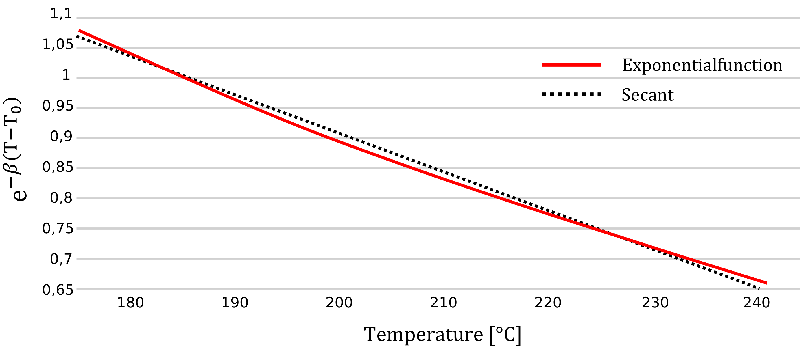
Image 1: approach of exponential function using a secant [Ang10]
In summary, the linearization with the Equation 10 produces the analytically solvable, simplified energy equation for the radial temperature (for $0 \leq \xi \leq 1$ and $0 \leq \zeta \leq 1$) [Ang10]:
$$\frac{\partial^2 \Theta}{\partial \xi^2} - Gz \frac{\partial \Theta}{\partial \xi} - c_2 \beta T_Z Br \Theta = -c_1 Br\tag{Equation 13}$$
The presented differential equation was successfully solved with the marginal conditions of the constant cylinder temperature and a tempered screw in the elaboration of [Sch13]. This model was adjusted according to the calculation of the temperature progression in the co-rotating twin screw extruder. As the solution contains dimensionless temperature data, these must still be converted into dimensioned data.
This can be done using the following equation and results in the ten data of the profile of the flight height.
$$T_{0,n}(\xi) = \theta_{\xi,n} T_{Z,n} + T_{n-1}\tag{Equation 14}$$
Finally the arithmetic mean is formed from the radial temperature data and the average canal temperature of the section is defined. Because of the step-by-step calculation in SIGMA the axial temperature curve can be calculated.
References
[1] Potente, H.: Rechnergestützte Extruderauslegung, Kunststofftechnisches Seminar, Paderborn, 1991.
[2] Koch, M.: Berechnung und Auslegung von Nutbuchsenextrudern, Dissertation, Universität Paderborn, 1987.
[3] Schulte, H.: Grundlagen zur verfahrenstechnischen Auslegung von Spritzgießplastifiziereinheiten, Dissertation, Universität Paderborn, 1990.
[4] Stenzel, H.; Ansahl, J.: Zur Temperaturberechnung in Ein- und Doppelschneckenextrudern, Universität Paderborn, 1990.
[5] Carslaw, H. S.; Jaeger, J. C.: Conduction of Heat in Solids, Oxford University Press, Oxford, 1959.
[6] Tadmor, Z.; Klein, I.: Engineering Principles of Plasticating Extrusion, Publishing Company, Huntington, NY, 1978.
[7] Melisch, U.: „Grundlagen zur Simulation des Förder- und Plastifizierprozesses dichtkämmender Gleichdrall-Doppelschneckenextruder“, Dissertation, Universität Paderborn, 1998.
[8] Ansahl, J.: Grundlagen für die Auslegung dichtkämmender Gleichdrall-Doppelschneckenextruder, Dissertation, Universität Paderborn, 1993.
[9] Mitterfellner, H.: Vergleich verschiedener Lösungen zur Analyse der Schmelzetemperaturentwicklung im Schneckenkanal von Einschneckenextrudern, Studienarbeit, Universität Paderborn, 1991.
[10] Stenzel, H.: Grundlagen zur Verfahrenstechnischen Auslegung von Barriereschnecken in Glattrohr- und Nutbuchsenextrudern, Dissertation, Universität Paderborn, 1992.
[11] Kretschmer, K.: Untersuchung und Beschreibung des Prozess- und Mischverhaltens von Mischelementen für Gleichdrall-Doppelschneckenextruder, Dissertation, Universität Paderborn, 2004.
[Ang10] Anger, K.: „Temperaturmodellierung von temperierten Einschnecken„; Dissertation am Institut für Kunststofftechnik (KTP); Universität Paderborn; 2010
[Sch13] Schadomsky, M.: „Weiterentwicklung eines mathematischen Modells zur Bestimmung der Temperaturverteilung intern temperierter Einschneckenextruder“; Studienarbeit am Institut für Kunststofftechnik (KTP) ; Universität Paderborn; 2013
[PS92] Potente H.; Schöppner V.: „Skript zur Vorlesung Rechnergestützte Extruderauslegung„; Institut für Kunststofftechnik (KTP); Universität Paderborn; 1992
[Kre04] Kretschmer, K.: „Untersuchung und Beschreibung des Prozess- und Mischverhaltens von Mischelementen für Gleichdrall-Doppelschneckenextruder“; Dissertation am Institut für Kunststofftechnik (KTP); Universität Paderborn; 2004