Dies ist eine alte Version des Dokuments!
Melt conveying
The basis of the general mathematical description of flow is the equilibrium of mass, momentum and energy. A flow is described, if at any place and at any time the velocity vector and the values pressure and temperature in the flow domain are known. For the calculation of these values, the conservative equations and the constitutive equations are combined [BSL60], [BAH77], [Böh81], [Jis82].
Isothermal flows in extruders are described by [Tuc89]:
1. The equilibrium of mass, $$\frac{\partial \rho}{\partial t} + \nabla \cdot (\rho \cdot v) = 0 \tag{1}$$ 2. the equilibrium of momentum $$\rho \frac{\delta v}{\delta t} = -\nabla p + \nabla \tau + \rho g \tag{2}$$ 3. and a rheological law $$\tau = \eta(\mathrm{II})\dot{\gamma} \tag{3}$$
Where $\rho$ is the melt density, p is the pressure, v is the velocity vector, $\tau$ is the shear stress tensor and D/Dt the total differential. $\eta(\mathrm{II})$ is the second invariant of the rate of deformation tensor.
The system of differential equation can be solved either analytically or numerically, depending on the degree of non-linearity within the system.
Linear Pressure Model and Polynomial Pressure Model
Conveying Elements and Kneading Blocks
Analytical Solution
The closed mathematical description of the general equations mentioned above requires restrictions of the system of differential equations by assumptions and boundary conditions.
For the models mentioned below we made the following prerequisites:
- The screw geometry can be described by a channel model
- The screw channel is completely full
- The flow is steady state and fully developed
- The flow is laminar
- The melt is incompressible
- In- and outflow effects are neglected
- The melt sticks to the wall
- Inertia terms are neglected
- Normal stresses are neglected
- Velocity components normal to the barrel wall are neglected
The analytical description of the melt conveying in co-rotating twin screw extruders is very complicated due to the self cleaning, tightly intermeshing screw profile. Since the profile is only defined piecewise. Because of this difficulty Ansahl [Ans93] replaced the real channel geometry by a rectangular channel with the same cross section.
In this section we will show a comparison of the flow in a real twin screw channel with that of a rectangular channel for a one-dimensional flow of a Newtonian fluid.

Figure: Coordinate system for the analysis of the melt conveying
Using the prerequisites mentioned above, the equilibrium of mass and the coordinate system shown in the figure, the momentum equation is reduced to:
$$-\frac{\partial p}{\partial z} - \eta \cdot \frac{\partial^2 v_z}{\partial y^2} = 0 \tag{4}$$
Solving this equation we get the velocity profile in the screw channel:
$$v_z(x,y) = \frac{1}{2\eta} \cdot \frac{\Delta p}{\Delta z}[y^2 + h(x) \cdot y] + v_{0z}\left[1 + \frac{y}{h(x)}\right] \tag{5}$$
With $v_{0z}$ being the velocity component in screw channel direction and h(x) the channel profile.
The velocity profile is not only dependent on the channel depth but also on the channel width, since the channel height of co-rotating twin screw extruder depends on the coordinate in the channel width direction.
Integrating eqn. 5 over the cross sectional area we get the flow rate:
$$\dot{V} = \int_{-\frac{b_{max}}{2}}^{\frac{b_{max}}{2}} \int_{-h(x)}^{0} v_z(x,y)dxdy \tag{6}$$
This integration can only be done analytically if h(x) = const. For twin screw channels this has to be done numerically.
By introducing a dimensionless throughput:
$$\pi_{\dot{V}} = \frac{\dot{V}}{\frac{1}{2}v_{0z}b_{max}\bar{h}} \tag{7}$$
and a dimensionless pressure gradient
$$\pi_p = \frac{\bar{h}^{1+n} \cdot \Delta p}{6Kv_{0z}^n \cdot Z} \tag{8}$$
a comparison of both channel geometries is made possible.
The figure shows the dimensionless throughput over the dimensionless pressure gradient for a one-dimensional flow of a Newtonian fluid. The profile for the rectangular channel intersects both axis at a value of 1.
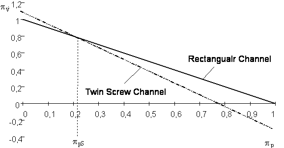
Figure: Pressure – throughput behavior of different channel profiles for a one dimensional flow of a Newtonian fluid.
The profile for the twin screw channel intersects the profile for the rectangular channel at the point $p_{pS}$. Below this point, in the area $\pi_p < \pi_{pS}$ higher dimensionless throughputs can be obtained. Above point $\pi_p < \pi_{pS}$ smaller dimensionless throughputs can be obtained in a twin screw channel.
Numerical Solution
The Finite Element Method (FEM) is an approximation method for the solution of differential equations. When applying this method, a continuum with infinite degrees of freedom is replaced by a set of finite elements with finite degrees of freedom [Chu82].
The description of the flow using the FEM is based as with the analytical solution, on the conservative equations. We used the FE program POLYFLOW [NN93] which was specially designed for the simulation of polymer flows. Flow problems can be either 2 dimensional, 2 ½ dimensional, 3 dimensional, steady state or transient. It is also possible to describe the flow behavior of polymer melts using different viscosity laws.
Analogous to the analytical solution, simplifications are needed to reduce the number of calculations. With the exception of the flow dimension, the same pre-requisites and simplifying assumptions were used to calculate the flow numerically as were used for the calculations shown above. Only in this instance we did not calculate a one dimensional flow but a 2 ½ dimensional flow. The figure shows the screw geometry of a single flighted, a double flighted and a triple flighted screw profile. For both the meshes used, the calculations and the stream lines are shown. We used a power law as a constitutive equation.

Figure: Meshes and streamlines for single, double and triple flighted screw elements.
The isothermal simulation calculation yields, given the duct volume flow rate, the multidimensional flow field and the pressure gradient established in the direction of the duct. Using the dimensionless parameters specified in the equations, the results can be expressed again in dimensionless form. The figure shows a comparison between a rectangular duct of the same cross-sectional area and a real twin-screw duct, considering a two-and-a-half-dimensional structurally viscous flow.
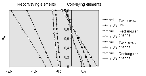
Figure: Pressure – throughput behavior of different channel profiles for a 2 ½ dimensional flow.
The analytical solution shows the intersecting profiles for the twin screw channel and the rectangular channel. A significant difference can be seen for reconveying elements.
As a result of these differences between the flow behavior in the real twin screw profile and in a rectangular channel it appears necessary to make a model that takes into account the real channel geometry.
Approximation - Model for the Calculation of Pressure Gradients
The Finite Element Method describes multi-dimensional flow fields. The applicability of this method is currently limited to the evaluation of certain screw sections. An overall simulation of one screw configuration is currently not possible.
The analytical description has the advantage of offering both simple and closed solutions. Due to the simplifications used for these models, differences between the real behavior and the model predictions can be observed.
To obtain a closed solution with an accurate level of prediction, we used the method of approximating the results of Finite Element simulations. The numerical results can be used for the calculation of machines which were not simulated, if the machine data is within the variation range of the data basis.
The dimensionless throughput and the dimensionless pressure gradient are related as follows:
$$\pi_V = f(\pi_P) \tag{9}$$
This relationship was investigated for different assumptions.
Potente [Pot83] investigated the 2 ½ dimensional flow in rectangular channels on the basis of numerical simulations. He found an approximation equation describing the pressure – throughput behavior. This approximation is based on a simple linear equation.
$$\pi_V = Y_1 - Y_2 \cdot \pi_P \tag{10}$$
The constants $Y_1$ and $Y_2$ take into account the transverse flow and the influence of the radial clearance.
The pressure – throughput diagram for the 2 ½ dimensional case is shown in Figure [Tad79] together with the prediction (dotted lines). The linear equation enables differences for low power law exponents to be observed.
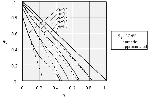
Figure: Dimensionless Flow Rate vs Dimensionless Pressure Gradient (2 dimensional flow in a rectangular channel) [Tad79]
Extended Approximation - Model for the Calculation of Pressure Gradients
The variation range of the influencing variables limits the scope of application for approximation equations. The influencing variables for co-rotating twin screw extruders are the number of flights $i$, the centerline ratio $CL = a/(D_S/2)$ , the ratio of pitch and screw diameter $t/D_S$ and finally the power law exponent $n$.
Conveying Screw Elements
For the Finite Element simulations the influencing variables varied in the following ways:
- Number of flights: $1 \leq i \leq 3$
- Pitch: $0.5 \leq t / D_S \leq 3$ (Conveying elements)
- $0.5 \leq t / D_S \leq 2$ (Reconveying elements)
- Centerline Ratio: $1.65 \leq CL \leq 1.85$
- Power Law Exponent: $0.2 \leq n \leq 1$
We used only those combinations which result into a tightly intermeshing screw profile. In total 14496 data points were achieved.
The resulting characteristic field was split into three sections. For each section an approximation equation was found.
Conveying element, $\pi_P \geq 0$:
$$\pi_V = c_{0P} + c_{1P} \cdot \pi_P + c_{2P} \cdot \pi_P^2 + c_{3P} \cdot \pi_P^3 \tag{11}$$
Conveying element, $\pi_P \leq 0$:
$$\pi_V = c_{0N} + c_{1N} \cdot \pi_P + c_{2N} \cdot \pi_P^3 + c_{3N} \cdot \pi_P^3 \tag{12}$$
Reconveying element, $\pi_P \geq 0$:
$$\pi_V = c_0 + c_1 \cdot \pi_P + c_2 \cdot \pi_P^2 \tag{13}$$
These equations were fitted to the characteristic profiles. The following boundary conditions were used for this fit:
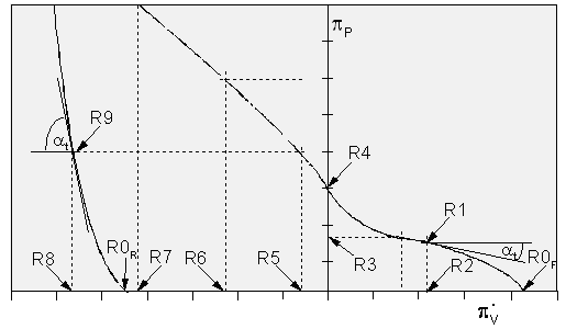
Figure: Position of the boundary conditions for conveying and reconveying elements
The figure shows the position of the boundary conditions used in the positive and the negative range of the dimensionless pressure gradient.
Boundary conditions for conveying elements ($\pi_P \geq 0$):
Boundary Condition 1: $\pi_P(\pi_V = 0) = \pi_{P0}$
Boundary Condition 2: Slope at the point of inflection $\pi_V'W$
Boundary Condition 3: Position of the point of inflection $\pi_{PW}$
Boundary Condition 4: $\pi_V(\pi_P = 0,15) = \pi_{V15}$
Boundary Condition 5: $\pi_V(\pi_P = 0) = \pi_{V0}$
Boundary conditions for conveying elements ($\pi_P \leq 0$):
Boundary Condition 1: $\pi_V(\pi_P = 0) = \pi_{V0}$
Boundary Condition 2: $\pi_P(\pi_V = 1,0) = \pi_{P10F}$
Boundary Condition 3: $\pi_P(\pi_V = 1,5) = \pi_{P15}$
Boundary Condition 4: $\pi_P(\pi_V = 2,0) = \pi_{P20}$
Boundary conditions for reconveying elements:
Boundary Condition 1: $\pi_P(\pi_V = 0) = \pi_{P0}$
Boundary Condition 2: $\pi_P(\pi_V = 1,0) = \pi_{P10R}$
Boundary Condition 3: $\pi'_V(\pi_V = 1,0) = \pi_{V'10}$
Since we were not able to obtain pressure throughput values for all boundary conditions, we had to take the missing values from equations that can be de-rived numerically. These boundary conditions are the slope at the point of inflection $\pi_V'W$, position of the point of inflection $\pi_{PW}$, the value for $\pi_{V0}$, the value for $\pi_P = 0,15$ ($\pi_{V15}$) and the value for $\pi_V = 1,0$ ($\pi_{V'10}$).
The quality of the approximation depends predominantly on the quality of the approximation of the boundary conditions. The influence of each variable was investigated individually. Due to this we found one equation for each variable. The actual approximation function was found by the recursive insertion of all equations into one another.
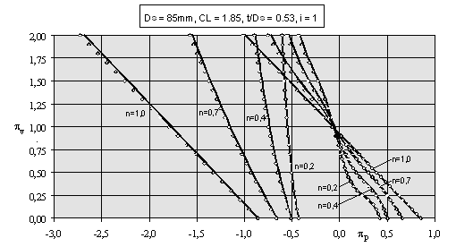
Figure: Comparison between approximated and numerical dimensionless pressure throughput behavior.
The figure provides an excellent comparison between the numerical data and the model predictions. The approximated characteristics (lines) were determined for the same flow rates as the numerical (symbols). The positive dimensionless pressure gradients show a good fit. Small differences between the model predictions and the numerical data can be found in the range of negative dimensionless pressure gradients. These differences, especially for power law exponents $n > 0.7$, can be explained by the chosen boundary conditions.
The figure shows the comparison of the model predictions, with the experimental data, which was obtained using polypropylene. In Figure the diagram is the same, although this time polystyrene was used. Both diagrams are plotted for three flighted conveying elements of a RZE 85.
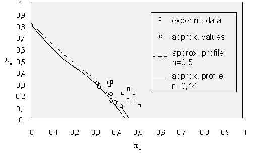
Figure: Comparison between experimental data and model predictions for a Polypropylene
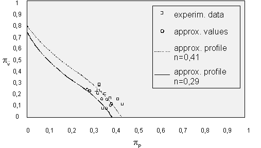
Figure: Comparison between experimental data and model predictions for a Polystyrene
The experimental data can be found close to or on the right hand side of the approximated line. The trend is basically the same. This means, that the model slightly underestimates the pressure build-up behavior of co-rotating twin screw extruders.
Leakage Flow
However, there are limitations in the production of the tightly intermeshing screw profile. Due to this there are clearances between the barrel and the screw flights. The material can flow in the neighboring channels. A model that takes into account the leakage flows was published in [Ans93].
In eqn. (14) equilibrium of flow rates for the channel model is shown.
$$\dot{V}_{ges} = k\dot{V}_z \mp \dot{V}_x \tag{14}$$
Where $\dot{V}_{ges}$ is the imposed flow rate to the system, $\dot{V}_z$ the flow rate in the channel and $\dot{V}_x$ the leakage flow rate, and k the number of parallel channels. The negative sign represents for conveying elements, the positive sign represents reconveying elements. Equation (14) can be rewritten in dimensionless form if it is divided by the drag flow rate.
$$\pi_{V,channel} = \pi_{V,z} \mp \pi_k\pi_{V,x} \tag{15}$$
with $p_k$ being a constant that takes into account the leakage length and the leakage height $s_R$.
$$\pi_k = \frac{(2\pi - \Omega)D_S \cos \varphi_S s_R \tan \varphi_S}{b_{max} \bar{h}} \tag{16}$$
For the description of the flow rate over the screw tip a one dimensional flow is assumed. This flow can be described by the following linear equation [Ans93]:
$$\pi_{\dot{V} ,x} = C_{0x} - C_{1x}\pi_P \tag{17}$$
the constants $C_{0x}$ and $C_{1x}$ depend on the screw element. For conveying elements eqn (18) can be used [Pot83]:
$$C_{0x} = 1 \qquad C_{1x} = \frac{1}{n^{0.94}} \tag{18}$$
for reconveying elements is used [NN93]:
$$C_{0x} = -\frac{(0.31 + 0.69n)}{n} e^{1-n} \qquad C_{1x} = \frac{1}{n}e^{1-n} \tag{19}$$
From these relationships we get a description for the pressure throughput relationship within a screw element:
Conveying element: $\pi_P \geq 0$:
$$\pi_{V,ges} = c_{0P} - \pi_k c_{0x} + (c_{1P} + \pi_k c_{1x}) \cdot \pi_P + c_{2P} \cdot \pi_P^2 + c_{3P} \cdot \pi_P^3 \tag{20}$$
Conveying element: $\pi_P \leq 0$:
$$\pi_{V,ges} = c_{0N} - \pi_k c_{0x} + (c_{1N} + \pi_k c_{1x})\pi_P + c_{2N}\pi_P^2 + c_{3N}\pi_P^3 \tag{21}$$
Reconveying element: $\pi_p \geq 0$:
$$\pi_{V,ges} = c_0 - \pi_k c_{0x} + (c_1 + \pi_k c_{1x})\pi_P + c_2\pi_P^2 \tag{22}$$
These equations are solved for the dimensionless pressure gradient. We take into account that there is more than one solution. As there is only one incorrect solution, it is very simple to determine.
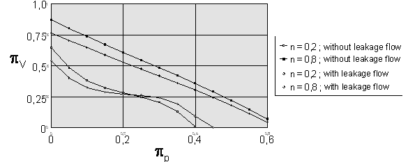
Figure: Comparison of the pressure-throughput characteristics with and without leakage flow for conveying elements
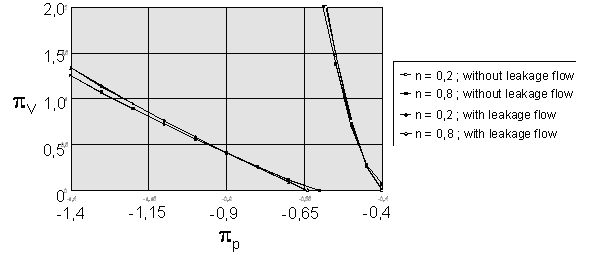
Figure: Comparison of the pressure-throughput characteristics with and without leakage flow for reconveying elements
The figures show the influence of the leakage flow on the dimensionless pressure throughput relationship for conveying and reconveying elements. The figures are based on the geometrical data of the ZSK 30 with a radial clearance of $s_R = 0.075$ mm and a pitch of 20 mm. The maximum influence of the leakage flow can be found at the point of $p_P = 0$ (pure drag flow). When $p_P$ is increased the influence of the leakage flow decreases. Due to the superposition of the polynomial equation for the channel flow and the linear equation for the leakage flow, the characteristic profiles intersect small power law exponents.
Neutral Kneading Blocks
Due to their conveying behavior, neutral kneading blocks are a special case. As the assembly of the kneading discs takes place at the staggering angle $\alpha=\pi/i$ there is no conveying direction. For the evaluation of the rheological behavior they must be regarded separately. This procedure is repeated for conveying elements.
The Finite Element simulations are based once again on those of the channel model. It is assumed that the pressure throughput behavior is the same as it would be for separate channels in series. With this assumption 2 ½ dimensional simulations are possible.
The figure shows the unwound channel geometry, together with the mesh used for the simulation
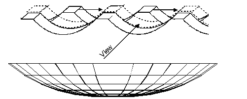
Figure: Finite Element mesh for neutral kneading blocks.
The results of the Finite Element simulations can be described by the dimensionless equation;
$$\pi_{PFN} = f(\pi_{\dot{V}FN}, n) \tag{23}$$
with the dimensionless throughput
$$\pi_{\dot{V}FN} = \frac{\dot{V}}{A_{channel}v_0} \tag{24}$$
and the dimensionless pressure gradient
$$\pi_{PFN} = \frac{A_{channel}^{\frac{1+n}{n}} \cdot \Delta p}{v_0^n K_{0T} \cdot L} \tag{25}$$
The figure clearly displays the results of the Finite Element Simulations (symbols) for different Power Law exponents n.
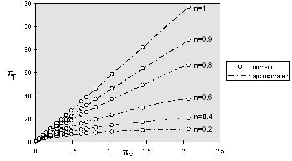
Figure: Pressure – throughput behavior of neutral kneading blocks
We get a linear relationship for a Power Law exponent n=1. The circulation flow has in this case no influence on the pressure throughput relationship. This case can be described by the equation:
$$\pi_{PFN,N} = \pi_\dot{V} \cdot (a_1 CL^3 + a_2 CL^2 + a_3) \tag{26}$$
Pseudoplastic materials can be described with the equation:
$$\pi_{PFN} = \pi_{PFN,N}^{n^{0,5}}(1 - n)\Delta\pi_P \tag{27}$$
with:
$$ \pi_P = \left(\pi_\dot{V} \frac{a_4}{CL^5} - a_5\right)\pi_\dot{V}^4 \frac{n}{CL^3} + \left(a_6n + a_7n^{\frac{1}{5}}CL^2 + \pi_\dot{V}^{\frac{3}{2}}a_8n^5CL^6\right)\pi_\dot{V}^{\frac{1}{2}}CL^4$$
$$+ \left[\left(\pi_\dot{V}^{2}a_9CL^{\frac{1}{2}} + a_{10}CL^4\right)\pi_\dot{V} + \pi_\dot{V}^n a_{11}n^4 + \pi_\dot{V}^{\frac{n}{5}}a_{12}\right]nCL \tag{28} $$
The constants $a_1$ to $a_{12}$ are shown in the table.
Table: Constants for the calculation of the dimensionless Pressure gradient for neutral kneading blocks
$a_1 = 370$ $a_2 = -873.733$ $a_3 = 2.49\pi^5$ $a_4 = 363$
$a_5 = -113$ $a_6 = 2.6$ $a_7 = -0.3083$ $a_8 = 1/22.5$
$a_9 = 13.3$ $a_{10} = -1.749$ $a_{11} = 2.928$ $a_{12} = 0.6589$
The range of validity of eqn. 28 depends on the centerline ratio.
For $CL \leq 1.75$
$$0 \leq \pi_{VFN} \leq 2 \tag{29}$$
and for $1.75 < CL \leq 1.85$:
$$0 \leq \pi_{VFN} \leq 3 \tag{30}$$
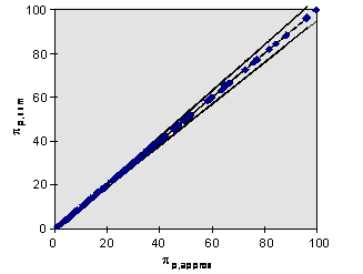
Figure: Comparison between approximated and numerical dimensionless pressure gradients for neutral kneading elements
The figure shows a comparison between the model predictions and the Finite Element results. The figure shows a scatter plot between the numerically determined results and the model predictions. From both figures we can see that the model is able to describe the numerically determined data.
The figure shows a comparison between the experimental determined data and the model predictions. The correlation is fairly good, especially if one considers the variance of the experimental data.
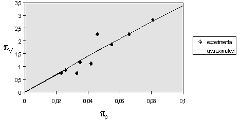
Figure: Comparison between approximated and experimental dimensionless pressure gradients for neutral kneading elements
Modelling of the Intermeshing Region
Diamond Shaped Channel
Using the channel model the complicated intermeshing region is replaced by a diamond shaped channel. Since the unwinding of the channel was carried out along the barrel surface, the intermeshing region is below the actual channel. A magnification of that region is shown in the figure.

Figure: Schematic diagram of the intermeshing region as a diamond shaped channel
The length $Z_{ei}$ in the figure is calculated using this equation:
$$Z_{ei} = \frac{L_{ei}}{\sin(\varphi_s)}\tag{31}$$
is calculated. The comparison, when considering the theoretical volumes $V_{fr1}$
$$A_r = A_{zw}L_{Ele}\tag{32}$$
with the theoretical volumes $V_{fr2}$ calculated according to the channel section flume model
$$V_{fr2} = k\bar{h}[b_{max}Z_{fr} + (b_{max}-e_{max})Z_{ei}]\tag{33}$$
shows deviations of less than approx. +/- 3 vol% for realistic ratios of centre-to-centre distance to screw outer diameter and a lead of up to $i = 3$, depending on the geometric conditions, i.e.:
$$V_{fr1} \approx V_{fr2}\tag{34}$$
By additionally incorporating the gusset as a channel constriction of length $Z_{ei}$ into the model, the resistance exerted by the gusset on the channel flow is taken into account. This gusset resistance is significant for single-start profiles, as large web widths are formed. For this reason, it must not be entirely disregarded when determining the flow rate characteristic curve.
Forced Conveying (Modified Model)
When performing three-dimensional flow simulations of twin screw elements one obtains a flow profile like the one shown in the figure. In this profile two different sections can be distinguished. Whereas in the intermeshing region quite high positive z-velocities can be found, in the channel region relatively low z-velocities are observed.
While there is apparently a backflow due to the pressure gradient in the channel region there is absolutely no backflow in the intermeshing region. This has to be taken into account for a model in the intermeshing region.
Due to the different flow patterns in the channel and in the intermeshing region, the different flows are modelled separately. From equilibrium of flow rates follows:
$$\dot{V}_{tot} = \dot{V}_{intermeshing area} + k \cdot \dot{V}_{channel} - \dot{V}_{gap} \tag{35}$$
The model for the flow rate in the intermeshing region assumes a chamber conveying in this region. This flow rate results from the volume in the intermeshing region and from the rotational speed.
$$\dot{V}_{intermeshing area} = \bar{V}_{intermeshing area} \cdot n_0 \tag{36}$$

Figure: Flow patterns in a conveying element (ZSK30, conveying element 28/28, PP Stamylan P17E19FC (DSM), V=2814mm³/s=7.53kg/h, no=455 1/min)
The calculation of the pressure – throughput relationship is carried out as described above. The only difference is, that the flow rate used for the calculation is not the flow rate imposed to the system but the imposed flow rate reduced by the flow rate in the intermeshing region.
Blister Elements
The calculation of the pressure gradients in blister elements is based on these simplifications:
- The gaps in the intermeshing region are equal ($s_{F1} \approx s_{F2}$).
- The geometry can be described as a series of discs (see figure).

Figure: Geometrical model for blister elements
The geometry can be characterized using the following dimensionless numbers:
$$k1 = \frac{D_i}{D_z} \tag{37}$$
$$k2 = \frac{D_i}{D_a} \tag{38}$$
$$cl = \frac{a}{D_z/2} \tag{39}$$
Analogous to the description of the pressure throughput relationship for conveying elements a dimensionless throughput,
$$\pi_V = \frac{\dot{V}}{0.5 \cdot A_{frei} \cdot D_a \cdot n_0} \tag{40}$$
a dimensionless pressure gradient
$$\pi_P = \frac{\Delta p \cdot R_z}{L \cdot n_0^n \cdot K} \tag{41}$$
and the Power Law exponent $n$ was used for the calculation.
For the Finite Element simulations the influencing variables varied as follows:
$k1$: $0.7 \leq k1 \leq 1$
$k2$: $0.7 \leq k2 \leq 0.98$
$Cl$: $1.65 \leq Cl \leq 1.85$
$n$: $0.2 \leq n \leq 1$
$\pi_V$: $0.01 \leq \pi_V \leq 5$
Since we used the power law for this model. The determination of the right average shear rate is crucial for the model. The shear rate is characterized by the dimensionless shear rate $\pi_{\dot{\gamma}}$.
$$\pi_\gamma = \left(\frac{\dot{\gamma}}{n_0}\right)^n \tag{42}$$
It depends on
- the geometry ($k1, k2, cl$)
- the dimensionless flow rate $\pi_V$
- the Power Law Exponent $n$
For the description we used a linear equation:
$$\pi_\gamma = A_0(k1, k2, cl, n) + A_1(k1, k2, cl, n) \cdot \pi_\gamma \tag{43}$$

Figure: Comparison of approximated and numerically determined dimensionless shear rates
The pressure throughput behavior can be described using the following polynomial equation:
$$\pi_V = A_{B,1}(k1, k2, cl, n) \cdot \pi_P + A_{B,2}(k1, k2, cl, n) \cdot \pi_P^2 \tag{44}$$
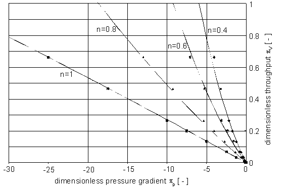
Figure: Comparison of approximated and numerically determined dimensionless flow rates
The pressure-flow rate behaviour can be approximated by a second-order polynomial:
$$\pi_V = A_{B,1}(k1, k2, cl, n) \cdot \pi_P + A_{B,2}(k1, k2, cl, n) \cdot \pi_P^2\tag{45}$$
A comparison of the pressure gradients predicted by the model with those determined experimentally shows sufficient agreement.
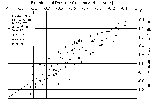
Figure: Comparison of approximated and experimentally determined pressure gradients
Turbine Mixing Elements
The following simplifications are made for the modelling of the turbine mixing elements:
- The gaps in the intermeshing region are equal ($s_{F1} \approx s_{F2}$).
- The flow in the grooves can be described by the flow in a similar rectangular channel

Figure: Real turbine mixing elements and the simplified model
Flow in the Grooves
The models describing the pressure throughput relationships in rectangular channels originate from the single screw theory. These equations can not be applied here since the width to height ratio is comparatively small and the pitch of the grooves is larger than the pitch usually used for single screw extruders. Furthermore one can find different conveying directions in turbine mixer elements. There are conveying, reconveying and neutral turbine mixer elements.
For the Finite Element simulations the influencing variables varied as follows:
- $b/h$: $0.05 \leq b/h \leq 40$
- $t/d$: $0.5 \leq t/d \leq 10$ (only conveying and reconveying)
- $n$: $0.2 \leq n \leq 1$
- $\pi_V$: $0 \leq \pi_V \leq 10$
The pressure throughput behavior of the three different flow directions can be described by the following polynomial equation:
$$\pi_V = A_{R,0} \left(\frac{t}{D_a}, \frac{b}{h}, n\right) + A_{R,1} \left(\frac{t}{D_a}, \frac{b}{h}, n\right) \cdot \pi_P + A_{R,2} \left(\frac{t}{D_a}, \frac{b}{h}, n\right) \cdot \pi_P^2 + A_{R,3} \left(\frac{t}{D_a}, \frac{b}{h}, n\right) \cdot \pi_P^3 \tag{46}$$
where the parameter $A_{R,0} = 0$ for neutral elements. In the figures the profiles of the dimensionless pressure gradients are shown.
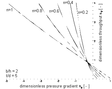
Figure: Comparison of approximated and numerically determined dimensionless flow rates for conveying rectangular channels
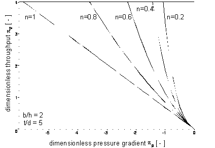
Figure: Comparison of approximated and numerically determined dimensionless flow rates for neutral rectangular channels
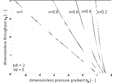
Figure: Comparison of approximated and numerically determined dimensionless flow rates for reconveying rectangular channels
Superposition of the Flow Rates
The pressure – throughput relationship of the turbine mixing element follows from the superposition of the flow rates in a comparable blister disc and the flow rates in the rectangular channels
$$\dot{V}_{tooth\ mixing\ element} = \dot{V}_{disc} + i \cdot \dot{V}_{rectangle} \tag{47}$$
The following equation describes the pressure throughput relationship for turbine mixing elements results from the above equation:
$$\pi_V = Y_0 + Y_1 \cdot \pi_P + Y_2 \cdot \pi_P^2 + Y_3 \cdot \pi_P^3 \tag{48}$$
with:
$$\pi_V = \frac{\dot{V}}{\frac{1}{2} \cdot n_0 \cdot A_{free} \cdot D_a} \tag{49}$$
$$\pi_P = \frac{\Delta p}{L} \cdot \frac{\overline{s_R}}{K \cdot n_0^n} \tag{50}$$
and
$$Y_0 = A_{R,0} \cdot i \cdot \pi_{geo,V}\tag{51}$$
$$Y_1 = A_{B,1} + A_{R,1} \cdot i \cdot \pi_{geo,V} \cdot \pi_{geo,p} \tag{52}$$
$$Y_2 = A_{B,2} + A_{R,2} \cdot i \cdot \pi_{geo,V} \cdot \pi_{geo,p}^2\tag{53}$$
$$Y_3 = A_{R,3} \cdot i \cdot \pi_{geo,V} \cdot \pi_{geo,p}^3\tag{54}$$
The coefficients $p_{geo,V}$ and $p_{geo,p}$ are combined to couple the flow rates and the pressure gradients. They are defined as follows:
$$\pi_{geo,V} = \frac{\frac{1}{2} \cdot h \cdot b \cdot v_{0z}}{\frac{1}{2} \cdot A_{free} \cdot D_a \cdot n_0} \tag{55}$$
and:
$$\pi_{geo,p} = \frac{h^{1+n}}{6 \cdot (\pi \cdot D_a \cdot \cos(\varphi_z))^n} \tag{56}$$
Depending on the conveying direction different pressure throughput behaviors are resulting (see figures).
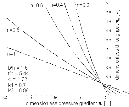
Figure: Pressure throughput behavior for conveying turbine mixing elements
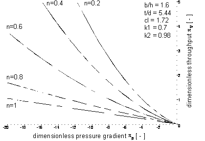
Figure: Pressure throughput behavior for neutral turbine mixing elements
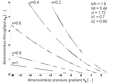
Figure: Pressure throughput behavior for reconveying turbine mixing elements
The comparison of the experimentally determined pressure differences and the predicted differences using a model show a significant correlation (see figure).
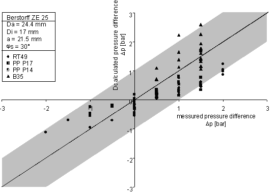
Figure: Comparison between experimentally determined data and the model predictions
Regression Model
Basis of the Flow Study in Screw Channels
The conservation laws for mass, momentum and energy are the basis of all mathematical-physical descriptions of flow processes. To describe a fact at any place at any time the velocity profile and the thermodynamical properties pressure, density and temperature have to be known. In addition, the conservation equation has to be connected with an equation to describe the material behavior. For solving the system with the help of conservation laws, additionally simplified assumptions have to be made and boundary conditions have to be given. The quality of the simplifications and the boundary conditions determine here the accuracy of the solution. All steps described above together form the physical-mathematical model.
Conservation laws
To describe the flow of polymer melts – as mentioned above – the conservation equations have to be solved. The conservation equations are here first generally given in differential form.
Continuity law
The continuity law is the mathematical formulation of a mass balance in a fixed control room. It states that the mass saved in a volume corresponds to the difference of inflowing and outflowing mass flows.
$$\frac{\partial \rho}{\partial t} + \nabla(\rho \cdot \vec{v}) = 0\tag{57}$$
Here $\rho$ is the density of the polymer melt, t the time and $\vec{v}$ the velocity vector.
Equation of motion (Principle of linear momentum)
The equation of motion is the difference between the momentum going in a volume element and that coming out of it plus the forces effecting the system (e.g. because of gravity).
$$\frac{\partial}{\partial t}(\rho \cdot \vec{v}) = -\nabla(\rho \cdot \vec{v} \cdot \vec{v}) - \nabla p - \nabla \tau + \rho \cdot \vec{a}\tag{58}$$
Law of conservation of energy
A formulation of the balancing of the heat quantity saved in the control room compared to inflowing and outflowing heat flows is the principle of conservation of energy.
$$\rho \cdot c \cdot \left(\frac{\partial T}{\partial t} + \vec{v} \cdot \nabla T\right) = -\nabla \vec{q} + \tau:\nabla \vec{v} + \phi\tag{59}$$
Materials law
With polymer melts the viscosity depends at the same time on the temperature and the shear rate. The literature describes models which model the single dependencies separately. Finally, the basic approaches are joined to a comprehensive description approach.
Most frequently used approaches to describe the shear rate dependency of the viscosity:
Power law $$\eta(\dot{\gamma}) = K \cdot a_T \cdot \dot{\gamma}^{n-1}\tag{60}$$
Carreau-approach $$\eta(\dot{\gamma}) = A \cdot a_T \cdot (1 + (B \cdot a_T \cdot \dot{\gamma})^c)^{-1}\tag{61}$$
Approach according to Carreau-Michaeli $$\eta(\dot{\gamma}) = A \cdot a_T \cdot (1 + B \cdot a_T \cdot \dot{\gamma})^{-c}\tag{62}$$
Yasuda-approach $$\eta(\dot{\gamma}) = A \cdot a_T \cdot (1 + (B \cdot a_T \cdot \dot{\gamma})^c)^{-\frac{c}{a}}\tag{63}$$
Approaches to describe the temperature dependency of the viscosity:
simplified Arrhenius-approach $$\ln(a_T) = -\beta \cdot (T - T_{ref})\tag{64}$$
Arrhenius-approach $$\ln(a_T) = -\frac{E}{R} \left(\frac{1}{T} - \frac{1}{T_{ref}}\right)\tag{65}$$
WLF-approach $$\log(a_T) = \frac{8.86 \cdot (T_{ref} - T_S)}{101.6 + T_{ref} - T_S} - \frac{8.86 \cdot (T - T_S)}{101.6 + T - T_S}\tag{66}$$
Mathematically the power law is easy to manage. Yet, using this approach has the advantage that this model is able to describe the flow behavior only in certain sections of the flow curve sufficiently well. A description of the whole flow curve in general with the help of this law is not possible. The first three approaches offer better descriptions. Yet, these have the advantage that they are mathematically difficult to manage. In the following the power law is used because of these disadvantages. Its parameter is locally adapted to the Carreau-Michaeli-law. The basis is that the average shear rate is known in the viewed flow section.
Finite element method to solve differential equations
The basis of the finite element simulations is the division of a continuum into infinitely many degrees of freedom due to finite elements with finitely many degrees of freedom [Chu89]. These elements are connected at nodes. The profiles of the functions searched for are described with trial functions which depict an approximation of the real profile. With the help of a suitable method the function values at the nodes are combined to a global equation system. Solving this system of equations is the main task of the finite element method. The accuracy can be improved by a smaller division of the continuum or by raising the degree of the trial function of the elements.
Modeling Procedure
The analysis of existing models to specify the pressure-throughput behavior of rectangular and twin screw flow channels gives evidence that these models are only suitable to a limited extent to describe mixing elements. This shall be explained on the basis of the results of a three-dimensional finite element simulation of a threaded-mixing element.
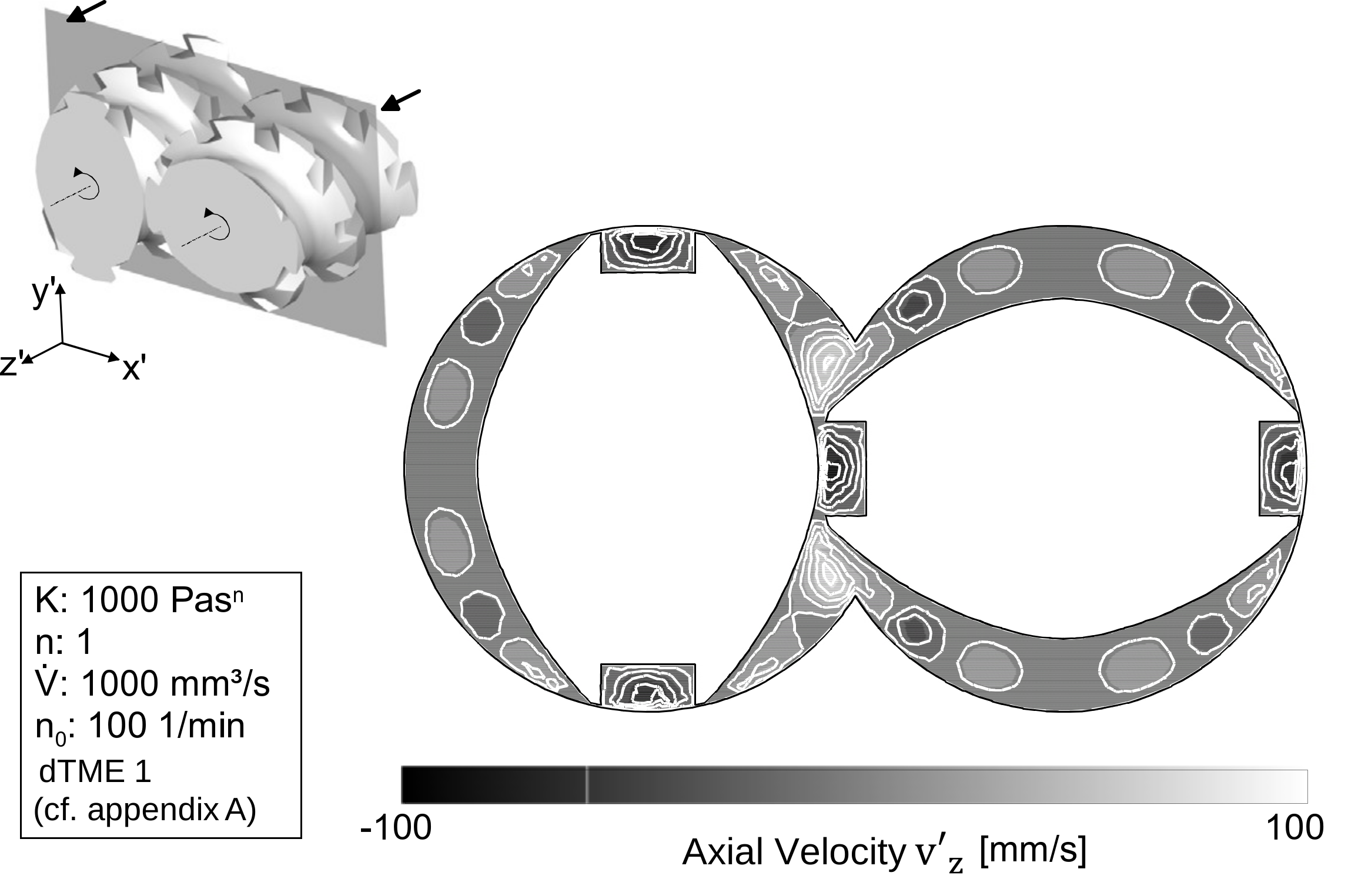
Figure: Velocity profiles in a threaded mixing element.
The figure illustrates the variation of the axial velocities in a conveying threaded mixing element with reconveying grooves.
It can be seen that negative axial velocities predominantly emerge in the area of the grooves. Correspondingly, the volume throughput in the grooves orientates in the opposite direction as the transport direction of the element. Deriving from this as well as from the geometries of the mixing elements the following requirements for pressure-throughput models are to be specified:
- areas, in which $\dot{V} \leq 0$, must be able to be represented,
- geometries, whose pitch to screw diameter ratio is $\frac{t}{D_s} > 2$, must be able to be incorporated and
- geometry sections, whose ratio of channel width to channel height is $\frac{b}{h} < 2$, must be able to be described.
Existing throughput equations for rectangular channels (e.g. [Jun00]) or for twin screw channels (e.g. [Ans93], [Mel00]) cannot fulfil these requirements.
To specify the throughput behavior of the screw elements, first of all, the basic geometry (twin screw channel, rectangular channel and disk elements) is analyzed and modelled. Subsequently, the models are superposed and integrated into an overall model for the description of the throughput behavior of the screw elements.
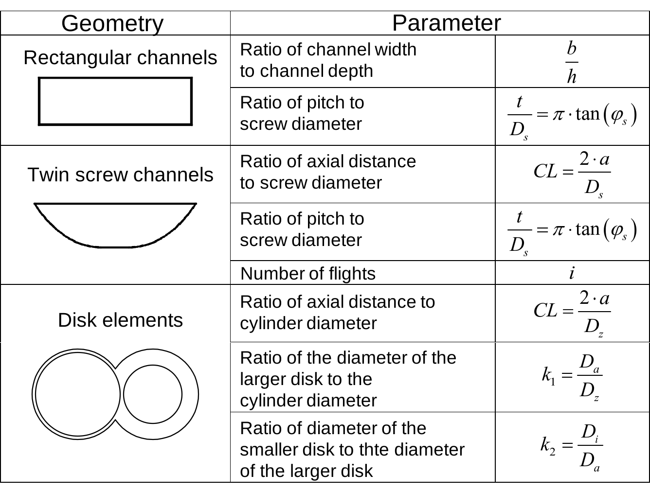 Table: Dimensionless parameters for the characterization of the geometry.
The data pool for the modelling was established on the basis of finite element simulations for all elements. To limit the amount of finite element calculations the geometry of the elements was standardized beforehand. The dimensionless parameters, which were utilized, are listed in the table.
In addition to the calculations the Power Law was applied. To restrict the error deriving from the application of the power law the pressure-throughput behavior as well as the shear rate were approximated. This enables the specification of the power law parameters in the interested shear rate area of the flow curve.
The presented models constitute approximations of the finite elements results. To attain physically sensible results certain boundary conditions are imposed on the model:
- The characteristic pressure-throughput curves are linear for Newton liquids.
- The models for the rectangular and the twin screw channels shall be applicable for conveying, reconveying and neutral channels.
For the modeling of the pressure-throughput behavior of rectangular channels the following boundary condition also has to be considered:
- In case of a Newtonian fluid (n=1), the influence of the helix angle on the pressure-throughput behavior decreases with an increasing ratio of b/h.
$$\pi_V = \left(\frac{b}{h} \rightarrow \infty, n = 1\right) = f(\varphi_s) \tag{67}$$
Due to the closely intermeshing geometry this requirement cannot be transferred to twin screw channels, because channel width and channel height can-not be varied independently. They are rather dependent on the pitch, the axial distance, the screw diameter, and the number of flights (see figure). Equation 67, however, can only be valid, if the channel width is independent of the pitch.

Figure: Influence of the helix angle on the geometry of twin screw channels.
For the modelling of the pressure-throughput behavior of the channel geometries the requirement of the applicability for conveying, reconveying and neutral channels implies, that the parameters applied by Ansahl [Ans93] and Melisch [Mel00] to specify the pressure-throughput behavior:
- the dimensionless volume throughput
$\pi_\dot{V} = \frac{\dot{V}}{\frac{1}{2} \cdot h \cdot b \cdot v_0 \cdot \cos(\varphi_s)}$
- the dimensionless pressure gradient
$\pi_p = \frac{\Delta p}{\Delta z} \cdot \frac{h^{1+n}}{6 \cdot K \cdot v_0^n \cdot \cos^n(\varphi_s)}$
are incompatible with this requirement, as they are not defined in the neutral case. On account of this, slightly modified parameters are used in these investigations.
$$\pi_\dot{V} = \frac{\dot{V}}{h \cdot b \cdot v_0} \tag{68}$$
and
$$\pi_p = \frac{\Delta p}{\Delta z} \cdot \frac{h^{1+n}}{K \cdot v_0^n} \tag{69}$$
To describe the process behavior of disk elements the following parameters are applied:
$$\pi_\dot{V} = \frac{\dot{V}}{A_{fr} \cdot D_a \cdot n_0} \tag{70}$$
$$\pi_p = \frac{\Delta p}{L} \cdot \frac{D_a}{K \cdot n_0^n} \tag{71}$$
The subsequent modelling of the pressure-throughput behavior of rectangular and twin screw channels shall form the basis of the modelling of the most diverse screw elements. The models of both channel types are based on the same procedure. The characteristic curve family can be separated into 3 sections (see figure).
- Section I: Here we observe a negative volume throughput. This can emerge in single channel areas; e.g. for grooved threaded elements a back-flow can be detected in the grooves.
- Section II: In this area a positive volume throughput and a positive pressure gradient are effective.
- Section III: In this area a negative pressure gradient and a positive volume throughput can be observed.

Figure: Boundary conditions for the modelling of the pressure-throughput behavior.
For a proper modelling special attention has to be paid to supply a sufficiently good description of the axis intercept points as depicted in the figure, as the partial models for the separate sections are linked with each other on the basis of these points. In the following the intersection point of the characteristic curve with the y-axis will be denominated as (dimensionless) drag conveying capacity. Physically this point represents a condition, in which the channel is completely filled but pressure is just not built up yet. The intersection point of the characteristic curve with the x-axis represents an operating point, in which the drag volume flow rates are as large as the volume flow rates, which arise from a pres-sure back stream. The consequence is that on aggregate there is no flow and that in such a way the examined channel area works as a closed mixing chamber.
The modelling of the pressure-throughput behavior is based upon a multitude of finite element simulations, in which the dimensionless parameters were varied systematically and completely factorial. The variation boundaries were selected in such a way that in part they clearly go beyond the hitherto technically realized spheres, so that a model extrapolation can be avoided as far as possible, which can always be problematic in statistical models. In detail, the parameters were varied within the boundaries as specified in the tables.
| Name | Formulaic symbol | Lower boundary | Upper boundary |
|---|---|---|---|
| Dimensionless throughput | $\pi_V$ | -6 | 6 |
| Dimensionless pressure gradient | $\pi_P$ | -18 | 18 |
| Exponent of the power law | $n$ | 0.2 | 1 |
| b/h ratio | $b/h$ | 0.4 | 40 |
| t/Ds ratio | $t/Ds$ | 0.2 | 10 |
Table: Variation of the parameters for the finite element simulations of rectangular channels.
| Name | Formulaic symbol | Lower boundary | Upper boundary |
|---|---|---|---|
| Dimensionless throughput | $\pi_V$ | -4 | 4 |
| Dimensionless pressure gradient | $\pi_P$ | -15 | 15 |
| Exponent of the power law | $n$ | 0.2 | 1 |
| Centerline Ratio | $CL$ | 1.5 | 1.85 |
| t/Ds ratio | $t/Ds$ | 0.2 | 5 |
| Number of flights | $i$ | 1 | 3 |
Table: Variation of the parameters for the finite element simulations of twin screw channels.
| Name | Formulaic symbol | Lower boundary | Upper boundary |
|---|---|---|---|
| Dimensionless throughput | $\pi_V$ | -4 | 4 |
| Dimensionless pressure gradient | $\pi_P$ | -15 | 15 |
| Exponent of the power law | $n$ | 0.2 | 1 |
| Centerline Ratio | $CL$ | 1.5 | 1.85 |
| Diameter ratio 1 | $k_1$ | 0.7 | 1 |
| Diameter ration 2 | $k_2$ | 0.7 | 0.98 |
Table: Variation of the parameters for the finite element simulations of disk elements.
Altogether, 61.727 finite element simulations resulted for rectangular channels, 94.392 simulations for twin screw channels and about 14.000 simulations for the disk elements.
Flow in Simple Geometries
Rectangular Channels
To describe the pressure-throughput behavior of rectangular channels the characteristic curve family is separated into three sections (see figure). For this, all those models were applied as specified in Eqs. 72 to 74. The parameters are dependent on the geometry and on the exponent of the power law. A detailed specification of the model equation can be found in the appendix C1.1 in [Kre04].
Section I: $$\pi_\dot{V} = \left(1 - \frac{\pi_p}{\pi_p|_{\pi_\dot{V}=0}}\right) \cdot \left(C_{RE,I,1} + C_{RE,I,2} \cdot \pi_p + C_{RE,I,3} \cdot \pi_p^2\right) \tag{72}$$
Section II: $$\pi_\dot{V} = \left(1 - \frac{\pi_p}{\pi_p|_{\pi_\dot{V}=0}}\right) \cdot \left(\pi_\dot{V}|_{\pi_p=0} + C_{RE,II,1} \cdot \pi_p + C_{RE,II,2} \cdot \pi_p^2\right) \tag{73}$$
Section III: $$\pi_\dot{V} = \pi_\dot{V}|_{\pi_p=0} + C_{RE,III,1} \cdot \pi_p + C_{RE,III,2} \cdot \pi_p^3 + +C_{RE,III,3} \cdot \pi_p^5 \tag{74}$$
with $$\pi_p|_{\pi_\dot{V}=0} = C_{Re,S,1} \cdot \cos(\varphi_s) + C_{Re,S,2} \cdot \cos^3(\varphi_s) + C_{Re,S,3} \cdot \cos^5(\varphi_s) \tag{75}$$
$$\pi_\dot{V}|_{\pi_p=0} = C_{Re,S,1} \cdot \cos(\varphi_s) + C_{Re,S,2} \cdot \cos^3(\varphi_s) + C_{Re,S,3} \cdot \cos^5(\varphi_s) \tag{76}$$
In the figure the calculated dimensionless pressure-throughput characteristics are contrasted with the Polyflow results of varying exponents of the power law. It can be seen, that the model offers a sufficiently good description for a wide area.

Figure: Comparison of the calculated and the predicted pressure-throughput characteristics for varying exponents of the power law.
The characteristic curves of conveying and reconveying channels are related to each other in a centrosymmetrical way
$$\pi_{\dot{V},FE}(\pi_{p,Fe}) = -\pi_{\dot{V},RFe}(-\pi_{p,RFe}) \tag{77}$$
i.e. if the characteristic curves of the conveying channels are known, those of the reconveying channels can be deduced from this basis.
The characteristic curve to specify the transportation neutral elements correspond with the specification in zone III, as the drag conveying capacity equals zero and as, therefore, the element is always overrun. The figure displays the pressure-throughput characteristics for the three types of transport and varying exponents of the power law. It can be recognized that the above outlined transformation of the characteristics allow a sufficiently good description of the Poly-flow results.

Figure: Comparison of the calculated and the predicted pressure-throughput characteristics of conveying, reconveying and neutral rectangular channels.
Twin Screw Channels
In an analogous way to the modelling procedure of rectangular channels in the modelling of twin screw channels also three areas can be separated (see figure). For the description of the particular zones all those models are used as specified in Eqs. 78 to 80. The parameters are dependent on the geometry and on the exponent of the power law. A detailed specification of the model equation can be found in the appendix C2.1 in [Kre04].
Section I: $$\pi_\dot{V} = \left(1 - \frac{\pi_p}{\pi_p|_{\pi_\dot{V}=0}}\right) \cdot \left(C_{DSE,I,1} + C_{DSE,I,2} \cdot \pi_p + C_{DSE,I,3} \cdot \pi_p^2\right) \tag{78}$$
Section II: $$\pi_\dot{V} = \left(1 - \frac{\pi_p}{\pi_p|_{\pi_\dot{V}=0}}\right) \cdot \left(C_{DSE,II,1} + C_{DSE,II,2} \cdot \pi_p + C_{DSE,II,3} \cdot \pi_p^2\right) \tag{79}$$
Section III: $$\pi_\dot{V} = \pi_\dot{V}|_{\pi_p=0} + C_{DSE,III,1} \cdot \pi_p + C_{DSE,III,2} \cdot \pi_p^3 + +C_{DSE,III,3} \cdot \pi_p^5 \tag{80}$$
with $$\pi_\dot{V}|_{\pi_p=0} = \frac{1}{C_{DSE,S,1} + C_{DSE,S,2} \cdot \overline{CL}} \tag{81}$$
$$\pi_p|_{\pi_\dot{V}=0} = \left(C_{DSE,P,1} + C_{DSE,P,2} \cdot \sqrt{CL}\right) \tag{82}$$
In the figure the dimensionless pressure-throughput characteristics are illustrated for varying exponents of the power law. It can be recognized that the model yields a sufficiently good description for a wide area.

Figure: Comparison of the calculated and the predicted pressure-throughput characteristics for varying exponents of the Power Law.
The description model of the throughput behavior of twin screw channels can be applied to conveying and reconveying channels. A comparison of the model predictions and the Polyflow results for both conveying and reconveying channels is illustrated in the figure. For all three transportation types a sufficiently good description can be identified.

Figure: Comparison of the calculated and the predicted pressure-throughput characteristics for conveying, reconveying and transportation neutral twin screw channels.
Disk Elements
Contrary to the previous geometries for the description of the throughput behavior of disk elements only one zone is examined. The motive for doing this is the fact that disk elements are neutral elements and, therefore, are always pressure consumers. Accordingly, a complete modelling can simply be attained on the basis of Section III of this element.
$$\pi_\dot{V} = C_{SE,1} \cdot \pi_p + C_{SE,2} \cdot \pi_p^2 + C_{SE,3} \cdot \pi_p^3 \tag{83}$$

Figure: Comparison of the calculated and the predicted pressure-throughput characteristics for varying exponents of the Power Law.
In the figure the dimensionless pressure-throughput characteristics are delineated for varying exponents of the power law. It can be recognized that the model gives a sufficiently good description for a wide area. The parameters in Equation 83 depend on the dimensionless geometry parameters as well as on the exponent of the power law. These are explained in detail in the appendix C3.1 in [Kre04].
Pressure-Throughput Model for Threaded Elements
In modeling the pressure-throughput behavior of threaded elements two distinct zones have to be differentiated, in which disparate mechanisms affect the transportation of the melt:
- transportation as a result of drag conveying mechanisms in the channel area and
- forced conveying in the intermeshing zone.
In the screw channels there can be observed insignificant, partly even negative, axial velocities. In the intermeshing zone of the screws, on the contrary, relatively high axial velocities are calculated. From this follows that at least for minor throughputs the transportation in the threaded element is dominated by the flow in the intermeshing zone. With these operating points a back-flow takes place in the screw channel.
To be able to represent this effect, first of all, the flow in the intermeshing zone and the flow in the screw channels are modelled separately before they are ultimately linked with each other.
$$\dot{V}_{GE} = \dot{V}_{intermeshing\ area,GE} + \dot{V}_{channel,GE} \tag{84}$$
Channel Area
For the description of the flow in the channel area a channel model is used, in which the screw and the barrel are uncoiled along the barrel wall. Additionally, a kinematic reversal is carried out, i.e. the rotating screw is represented by stationary, parallel channels above which moves the unwounded barrel (see figure).

Figure: Conveyor channel model for double-flighted conveying threaded elements [Ans93]
The velocity $v_0$ of the uncoiled barrel (see figure) equals the peripheral velocity at the outside diameter of the screw, which rotates with a speed of $n_0$.
$$v_0 = \pi \cdot D_s \cdot n_0 \tag{85}$$
The modeling of the throughput behavior is now based on a volume flow balance at the control rooms ABC in Figure.
$$\dot{V}_{channel,GE} = k \cdot \dot{V}_{z,GE} + \dot{V}_{x,GE} \tag{86}$$
Flow in the Channel
For the description of the flow in the conveyor channel $\dot{V}_z$ the approach specified in chapter is applied.
$$\dot{V}_{z,GE} = \pi_{V,z,GE} \cdot (\overline{h} \cdot b_{max} \cdot v_0) \tag{87}$$
It has to be taken into consideration that the calculation of $\pi_{V,z}$ is performed in sections:
$$\pi_{V,z,GE} = \begin{cases} \left(1 - \frac{\pi_{p,z}}{\pi_{p,z}|_{\pi_V=0}}\right) \cdot \left(C_{DSE,I,1} + C_{DSE,I,2} \cdot \pi_{p,z} + C_{DSE,I,3} \cdot \pi_{p,z}^2\right) & \pi_{V,z} < 0 \\ \left(1 - \frac{\pi_{p,z}}{\pi_{p,z}|_{\pi_V=0}}\right) \cdot \left(\pi_V|_{\pi_{p,z}=0} + C_{DSE,II,1} \cdot \pi_{p,z} + C_{DSE,II,2} \cdot \pi_{p,z}^2\right) & \text{für } 0 \leq \pi_{V,z} \leq \pi_V|_{\pi_{p,z}=0} \\ \pi_V|_{\pi_{p,z}=0} + C_{DSE,III,1} \cdot \pi_{p,z} + C_{DSE,III,2} \cdot \pi_{p,z}^3 + +C_{DSE,III,3} \cdot \pi_{p,z}^5 & \pi_V|_{\pi_{p,z}=0} \leq \pi_{V,z} \end{cases} \tag{88}$$
with
$$\pi_{p,z} = \frac{\Delta p}{Z_{Tv}} \cdot \frac{\overline{h}^{1+n}}{K \cdot v_0^n} \tag{89}$$
Accordingly, for the following measures it appears appropriate to formulate Equation 88 in a general form:
$$\pi_{\dot{V},z,GE} = A_{DSE,0} + A_{DSE,1} \cdot \pi_{p,z} + A_{DSE,2} \cdot \pi_{p,z}^2 + A_{DSE,3} \cdot \pi_{p,z}^3 + A_{DSE,4} \cdot \pi_{p,z}^5 \tag{90}$$
Flow in the Radial Clearance
For the description of the leakage flow $\dot{V}_x$ the approach for rectangular channels is used as specified in Chapter Flow in the Channel.
$$\dot{V}_{x,GE} = \pi_{V,x} \cdot (s_R \cdot b_{flight} \cdot v_0) \tag{91}$$
It has to be taken into consideration that the calculation of $\pi_{V,x}$ is performed in sections:
$$\pi_{V,x,GE} = \begin{cases} \left(1 - \frac{\pi_{p,x}}{\pi_{p,x}|_{\pi_V=0}}\right) \cdot \left(C_{RE,I,1} + C_{RE,I,2} \cdot \pi_{p,x} + C_{RE,I,3} \cdot \pi_{p,x}^2\right) & \pi_{V,x} < 0 \\ \\ \left(1 - \frac{\pi_{p,x}}{\pi_{p,x}|_{\pi_V=0}}\right) \cdot \left(\pi_V|_{\pi_{p,x}=0} + C_{RE,II,1} \cdot \pi_{p,x} + C_{RE,II,2} \cdot \pi_{p,x}^2\right) & \text{für } 0 \leq \pi_{V,x} \leq \pi_V|_{\pi_{p,x}=0} \\ \\ \left(\pi_V|_{\pi_{p,x}=0} + C_{RE,III,1} \cdot \pi_{p,x} + C_{RE,III,2} \cdot \pi_{p,x}^3 + +C_{RE,III,3} \cdot \pi_{p,x}^5\right) & \pi_V|_{\pi_{p,x}=0} \leq \pi_{V,x} \end{cases}\tag{92}$$
with
$$\pi_{p,x} = \frac{\Delta p}{e_{max}} \cdot \frac{s_R^{1+n}}{K \cdot v_0^n} \tag{93}$$
By virtue of clarity a general notation is also chosen:
$$\pi_{\dot{V},x} = A_{RE,0} + A_{RE,1} \cdot \pi_{p,x} + A_{RE,2} \cdot \pi_{p,x}^2 + A_{RE,3} \cdot \pi_{p,x}^3 + A_{RE,4} \cdot \pi_{p,x}^5 \tag{94}$$
Linkage of the Volume Flow Rates
If we solve the equations for the dimensionalised volume flows and then substitute these back in, we obtain:
$$\dot{V}_{channel,GE} = k \cdot (\overline{h} \cdot b_{max} \cdot v_0) \cdot (A_{DSE,0} + A_{DSE,1} \cdot \pi_{p,z} + A_{DSE,2} \cdot \pi_{p,z}^2$$ $$+ A_{DSE,3} \cdot \pi_{p,z}^3 + A_{DSE,4} \cdot \pi_{p,z}^5) + (s_R \cdot b_{steg} \cdot v_0) \cdot (A_{RE,0}$$ $$+ A_{RE,1} \cdot \pi_{p,x} + A_{RE,2} \cdot \pi_{p,x}^2 + A_{RE,3} \cdot \pi_{p,x}^3 + A_{RE,4} \cdot \pi_{p,x}^5) \tag{95}$$
Is this equation standardized to $k \cdot (\overline{h} \cdot b_{max} \cdot v_0)$, then follows:
$$\pi_{V,GE} = \frac{\dot{V}_{channel,GE}}{k \cdot (\overline{h} \cdot b_{max} \cdot v_0)} = (A_{DSE,0} + A_{DSE,1} \cdot \pi_{p,z} + A_{DSE,2} \cdot \pi_{p,z}^2$$ $$+ A_{DSE,3} \cdot \pi_{p,z}^3 + A_{DSE,4} \cdot \pi_{p,z}^5) + \frac{(s_R \cdot b_{steg} \cdot v_0)}{k \cdot (\overline{h} \cdot b_{max} \cdot v_0)} \cdot (A_{RE,0}$$ $$+ A_{RE,1} \cdot \pi_{p,x} + A_{RE,2} \cdot \pi_{p,x}^2 + A_{RE,3} \cdot \pi_{p,x}^3 + A_{RE,4} \cdot \pi_{p,x}^5)\tag{96}$$
As a next measure it proves necessary to build a linkage of the pressure gradients in channel direction and above the screw flight. For this purpose the approach proposed by Ansahl [Ans93] is reverted to. According to Ansahl the following equation applies:
$$\Delta p_x = \frac{\Delta p \cdot b_{max} + e_{max}}{\tan(\varphi_s)} \tag{97}$$
$$\pi_{p,x} = \frac{\Delta p \cdot b_{max} + e_{max} \cdot s_R^{1+n}}{\Delta z \cdot e_{max} \cdot \tan(\varphi_s) \cdot K \cdot v_0^n} = \pi_{geo,GE} \cdot \pi_{p,z} \tag{98}$$
$$\pi_{geo,GE} = \frac{b_{max} + e_{max}}{e_{max} \cdot \tan(\varphi_s)} \cdot \left(\frac{s_R}{\overline{h}}\right)^{1+n} \tag{99}$$
This gives us the equation for calculating the pressure-flow rate behaviour of the channel section of threaded elements for twin-screw extruders: $$\pi_{V,GE} = \left(A_{DSE,0} + \pi_1 \cdot A_{RE,0}\right)$$ $$+ \left(A_{DSE,1} + \pi_1 \cdot \pi_{geo} \cdot A_{RE,1}\right) \cdot \pi_{p,z}$$ $$+ \left(A_{DSE,2} + \pi_1 \cdot \pi_{geo}^2 \cdot A_{RE,2}\right) \cdot \pi_{p,z}^2$$ $$+ \left(A_{DSE,3} + \pi_1 \cdot \pi_{geo}^3 \cdot A_{RE,3}\right) \cdot \pi_{p,z}^3$$ $$+ \left(A_{DSE,4} + \pi_1 \cdot \pi_{geo}^5 \cdot A_{RE,4}\right) \cdot \pi_{p,z}^5 \tag{100}$$
with
$$\pi_1 = \frac{(s_R \cdot b_{steg} \cdot v_0)}{k \cdot (\overline{h} \cdot b_{max} \cdot v_0)} \tag{101}$$
Intermeshing Zone
In the literature diverse approaches to describe the flow in the intermeshing zone have been developed. In the following the approach of Booy [Boo80] is used.
$$\dot{V}_{intermeshing\ area,GE} = A_{intermeshing\ area} \cdot t \cdot n_0 \tag{102}$$
On the basis of measurements and flow simulations Bakalis [BK02] demonstrated, that the volume flow rates are well concordant with the measurements and the simulation results.
Pressure - Throughput Model
As a final step the volume throughput in the conveyor channel model is to be superposed with the volume throughput in the intermeshing zone:
$$\dot{V}_{GE} = \dot{V}_{intermeshing,GE} + \dot{V}_{channel,GE} = \dot{V}_{intermeshing\ area,GE} + \pi_{V,channel,GE} \cdot (\overline{h} \cdot b_{max} \cdot v_0) \tag{103}$$
In the figure the theoretical pressure-throughput characteristics are illustrated for conveying and reconveying threaded elements.

Figure: Pressure-throughput behavior of conveying and reconveying threaded elements.
In the figure the model predictions are compared with the experimental results. The experiments were performed with a model extruder using silicon oil as melt.

Figure: Comparison of calculated and measured pressure gradients in threaded elements.
It can be recognized that the model can offer a sufficiently good description of the measured pressure gradients.
Pressure-Throughput Model for Closely Intermeshing Threaded Mixing Elements
In the figure the variation of the axial velocities in a conveying, closely intermeshing thread mixing element are illustrated on two different levels. Out of the variation of the velocities it can be noticed that the flow in the grooves and in the intermeshing zone of both screws significantly differs from the flow in the channel area. In the intermeshing zone axial velocities can be detected, which are considerably higher than those in the channel area. In the grooves, however, another effect can be observed. As the grooves are of a back-flow design (in this case), in this area a back-flow is to be recognized accordingly. In the modelling, at first, a distinction is made between the intermeshing zone and the channel zone.
$$\dot{V}_{dGME} = \dot{V}_{channel,dGME} + \dot{V}_{intermeshing\ area,dGME} \tag{104}$$
The influence of the grooves on the behavior of the elements is then taken account of in the description of the separate areas.

Figure: Calculated velocity fields in a tightly intermeshing threaded mixing element.
Channel Model for the Channel Area
The channel model for tightly intermeshing threaded mixing elements can be compared to that of threaded elements. The flow in the grooves was accounted for by an additional volume throughput in the balance 105 of the marked control room ABC illustrated in see figure.

Figure: Channel model for a reconveying, intermeshing threaded mixing element.
A volume flow balance in the control room as depicted in the figure results in the following equation:
$$\dot{V}_{channel,dGME} = k \cdot \dot{V}_{z,dGME} + \dot{V}_{x,dGME} + l \cdot \dot{V}_{groove,dGME} \tag{105}$$
For the description of the flow in channel direction and in the grooves all models developed in chapter Rectangular channels and chapter Twin Screw Channels respectively are used in a general form:
$$\pi_{\dot{V},z,dGME} = A_{DSE,0} + A_{DSE,1} \cdot \pi_{p,z} + A_{DSE,2} \cdot \pi_{p,z}^2 + A_{DSE,3} \cdot \pi_{p,z}^3 + A_{DSE,4} \cdot \pi_{p,z}^5 \tag{106}$$
$$\pi_{\dot{V},x,dGME} = A_{RE,0} + A_{RE,1} \cdot \pi_{p,x} + A_{RE,2} \cdot \pi_{p,x}^2 + A_{RE,3} \cdot \pi_{p,x}^3 + A_{RE,4} \cdot \pi_{p,x}^5\tag{107}$$
$$\pi_{\dot{V},groove,dGME} = A_{RE,N,0} + A_{RE,N,1} \cdot \pi_{p,N} + A_{RE,N,2} \cdot \pi_{p,N}^2 + A_{RE,N,3} \cdot \pi_{p,N}^3 + A_{RE,4} \cdot \pi_{p,N}^5\tag{108}$$
with
$$\dot{V}_{z,dGME} = \pi_{\dot{V},z} \cdot (\bar{h} \cdot b_{max} \cdot v_0) \tag{109}$$
$$\dot{V}_{x,dGME} = \pi_{\dot{V},x} \cdot (h_N \cdot b_N \cdot v_0)\tag{110}$$
$$\dot{V}_{groove,dGME} = \pi_{\dot{V},N} \cdot (h_N \cdot b_N \cdot v_0)\tag{111}$$
and
$$\pi_{p,z} = \frac{\Delta p}{\Delta z} \cdot \frac{\bar{h}^{1+n}}{K \cdot v_0^n} \tag{112}$$
$$\pi_{p,x} = \frac{\Delta p}{x} \cdot \frac{s_R^{1+n}}{K \cdot v_0^n} \tag{113}$$
$$\pi_{p,N} = \frac{\Delta p}{x} \cdot \frac{h_N}{K \cdot v_0^n} \tag{114}$$
and
$$\pi_{\dot{V},z,dGME} = \frac{\dot{V}_z}{\bar{h} \cdot b_{max} \cdot v_0} \tag{115}$$
$$\pi_{\dot{V},x,dGME} = \frac{\dot{V}_x}{s_R \cdot b_{Steg} \cdot v_0} \tag{116}$$
$$\pi_{\dot{V},x,dGME} = \frac{\dot{V}_{Nut}}{h_N \cdot b_N \cdot v_0} \tag{117}$$
Substituting gives:
$$\dot{V}_{channel,dGME} = k \cdot (\bar{h} \cdot b_{max} \cdot v_0) \cdot A_{DSE,0} + (A_{DSE,1} \cdot \pi_{p,z} + A_{DSE,2} \cdot \pi_{p,z}^2$$
$$+A_{DSE,3} \cdot \pi_{p,z}^3 + A_{DSE,4} \cdot \pi_{p,z}^5) + (s_R \cdot b_{steg} \cdot v_0) \cdot (A_{RE,0}$$
$$+A_{RE,1} \cdot \pi_{p,x} + A_{RE,2} \cdot \pi_{p,x}^2 + A_{RE,3} \cdot \pi_{p,x}^3 + A_{RE,4} \cdot \pi_{p,x}^5)$$
$$+l \cdot (h_N \cdot b_N \cdot v_0) \cdot (A_{RE,N,0} + A_{RE,N,1} \cdot \pi_{p,N} + A_{RE,N,2} \cdot \pi_{p,N}^2$$
$$+A_{RE,N,3} \cdot \pi_{p,N}^3 + A_{RE,4} \cdot \pi_{p,N}^5)\tag{118}$$
Is this equation standardized to $k \cdot (\bar{h} \cdot b_{max} \cdot v_0)$, then follows:
$$\pi_{\dot{V},channel,dGME} = \frac{\dot{V}_{channel,dGME}}{k \cdot (\bar{h} \cdot b_{max} \cdot v_0)} = A_{DSE,0} + (A_{DSE,1} \cdot \pi_{p,z} + A_{DSE,2} \cdot \pi_{p,z}^2$$
$$+A_{DSE,3} \cdot \pi_{p,z}^3 + A_{DSE,4} \cdot \pi_{p,z}^5) + \frac{(s_R \cdot b_{thread} \cdot v_0)}{k \cdot (\bar{h} \cdot b_{max} \cdot v_0)} \cdot (A_{RE,0}$$
$$+A_{RE,1} \cdot \pi_{p,x} + A_{RE,2} \cdot \pi_{p,x}^2 + A_{RE,3} \cdot \pi_{p,x}^3 + A_{RE,4} \cdot \pi_{p,x}^5) $$
$$+ \frac{l \cdot (h_N \cdot b_N \cdot v_0)}{k \cdot (\bar{h} \cdot b_{max} \cdot v_0)} \cdot (A_{RE,N,0} + A_{RE,N,1} \cdot \pi_{p,N} + A_{RE,N,2} \cdot \pi_{p,N}^2$$
$$+A_{RE,N,3} \cdot \pi_{p,N}^3 + A_{RE,4} \cdot \pi_{p,N}^5)\tag{119}$$
To obtain a comprehensive description of the process behavior the pressure gradient in conveyor channel direction is to be linked with the pressure gradients above the radial clearance and with the pressure gradient in the groove. For this purpose the approach proposed by Ansahl [Ans93] is reverted to (see chap. Linkage of the Volume Flow Rates). The linkage of the pressure gradients in the conveyor channel and in the groove can be carried out analogously. It only has to be taken into account that the grooves are inserted in a specific angle in the screw flank, so that the length, in which the pressure gradient is effective, in the grooves differs from the length of the screw flight. Consequently, the pressure gradients can be interlinked as follows.
$$\pi_{p,x} = \frac{\Delta p}{\Delta z} \cdot \frac{b_{max} + e_{max}}{e_{max} \cdot \tan(\varphi_s)} \cdot \frac{s_R^{1+n}}{K \cdot v_0^n} = \pi_{geo,GE} \cdot \pi_{p,z}\tag{120}$$
$$\pi_{p,N} = \frac{\Delta p}{\Delta z} \cdot \frac{b_{max} + e_{max}}{e_{max} \cdot \tan(\varphi_s)} \cdot \cos\left(\frac{\pi}{2} - \varphi_s - \varphi_N\right) \cdot \frac{h_N^{1+n}}{K \cdot v_0^n} = \pi_{geo,N} \cdot \pi_{p,z}\tag{121}$$
$$\pi_{p,x} = \frac{\Delta p}{\Delta z} \cdot \frac{b_{max} + e_{max}}{e_{max} \cdot \tan(\varphi_s)} \cdot \frac{s_R^{1+n}}{K \cdot v_0^n} = \pi_{geo,x} \cdot \pi_{p,z}\tag{122}$$
$$\pi_{p,N} = \frac{\Delta p}{\Delta z} \cdot \frac{b_{max} + e_{max}}{e_{max} \cdot \tan(\varphi_s)} \cdot \cos\left(\frac{\pi}{2} - \varphi_s - \varphi_N\right) \cdot \left(\frac{h_N}{\bar{h}}\right)^{1+n} = \pi_{geo,N} \cdot \pi_{p,z}\tag{123}$$
with:
$$\pi_{geo,GE} = \frac{b_{max} + e_{max}}{e_{max} \cdot \tan(\varphi_s)} \cdot \left(\frac{s_R}{\bar{h}}\right)^{1+n}\tag{124}$$
$$\pi_{geo,N} = \frac{\Delta p \cdot b_{max} + e_{max}}{\Delta z \cdot e_{max} \cdot \tan(\varphi_s)} \cdot \cos\left(\frac{\pi}{2} - \varphi_s - \varphi_N\right) \cdot \left(\frac{h_N}{\bar{h}}\right)^{1+n}\tag{125}$$
From the equations, we obtain:
$$\pi_{ \dot V,Kanal,dGME} = \left(A_{DSE,0} + A_{DSE,1} \cdot \pi_{p,z} + A_{DSE,2} \cdot \pi_{p,z}^2 + A_{DSE,3} \cdot \pi_{p,z}^3\right.$$ $$\left.+A_{DSE,4} \cdot \pi_{p,z}^5\right) + \pi_1 \cdot \left(A_{RE,0} + A_{RE,1} \cdot \left(\pi_{p,z} \cdot \pi_{geo}\right)\right.$$ $$\left.+A_{RE,2} \cdot \left(\pi_{p,z} \cdot \pi_{geo}\right)^2 + A_{RE,3} \cdot \left(\pi_{p,z} \cdot \pi_{geo}\right)^3 + A_{RE,4} \cdot \left(\pi_{p,z} \cdot \pi_{geo}\right)^5\right)$$ $$+\pi_2 \cdot \left(A_{RE,N,0} + A_{RE,N,1} \cdot \left(\pi_{p,z} \cdot \pi_{geo,N}\right) + A_{RE,N,2} \cdot \left(\pi_{p,z} \cdot \pi_{geo,N}\right)^2\right.$$ $$\left.+A_{RE,N,3} \cdot \left(\pi_{p,z} \cdot \pi_{geo,N}\right)^3 + A_{RE,N,4} \cdot \left(\pi_{p,z} \cdot \pi_{geo,N}\right)^5\right)\tag{126}$$
with
$$\pi_1 = \frac{\left(s_R \cdot b_{Steg} \cdot v_0\right)}{k \cdot \left(\bar{h} \cdot b_{max} \cdot v_0\right)}\tag{127}$$
$$\pi_2 = \frac{l \cdot \left(h_N \cdot b_N \cdot v_0\right)}{k \cdot \left(\bar{h} \cdot b_{max} \cdot v_0\right)}\tag{128}$$
the equation for calculating the pressure-flow characteristics of the channel section of threaded elements:
$$\pi_{\dot V,GE} = \left(A_{DSE,0} + \pi_1 \cdot A_{RE,0} + \pi_2 \cdot A_{RE,N,0}\right)$$ $$+\left(A_{DSE,1} + \pi_1 \cdot \pi_{geo} \cdot A_{RE,1} + \pi_2 \cdot \pi_{geo,N} \cdot A_{RE,N,1}\right) \cdot \pi_{p,z}$$ $$+\left(A_{DSE,2} + \pi_1 \cdot \pi_{geo}^2 \cdot A_{RE,2} + \pi_2 \cdot \pi_{geo,N}^2 \cdot A_{RE,N,2}\right) \cdot \pi_{p,z}^2$$ $$+\left(A_{DSE,3} + \pi_1 \cdot \pi_{geo}^3 \cdot A_{RE,3} + \pi_2 \cdot \pi_{geo,N}^3 \cdot A_{RE,N,3}\right) \cdot \pi_{p,z}^3$$ $$+\left(A_{DSE,4} + \pi_1 \cdot \pi_{geo}^5 \cdot A_{RE,4} + \pi_2 \cdot \pi_{geo,N}^5 \cdot A_{RE,N,4}\right) \cdot \pi_{p,z}^5\tag{129}$$
Intermeshing Zone
The flow in the intermeshing zone is made up of a proportion of chamber transport and a transport in the grooves (see figure).
For the description of the throughput behavior in the intermeshing zone it is assumed that the throughput behavior is substantially dominated by a chamber flow. The grooves in the intermeshing zone alone result in an influence of the pressure gradient on the flow.
$$\dot{V}_{intermeshing\,area,dGME} = \overline A_{intermeshing\,area} \cdot t \cdot n_0 + l_{zw} \cdot \pi_{V,intermeshing\,area} \cdot (h_N \cdot b_N \cdot v_{zw}) \tag{130}$$
To specify the groove flow the description of the rectangular channels is applied:
$$\pi_{\dot{V},intermeshing,dGME} = A_{RE,Z,0} + A_{RE,Z,1} \cdot \pi_{p,zw} + A_{RE,Z,2} \cdot \pi_{p,zw}^2 + A_{RE,Z,3} \cdot \pi_{p,zw}^3 + A_{RE,Z,4} \cdot \pi_{p,zw}^5 \tag{131}$$

Figure: Axial velocities in the intermeshing zone of a closely intermeshing threaded mixing element.
For the linkage of the pressure gradients in the intermeshing zone and in the conveyor channel area it is assumed that the back pressure in the intermeshing zone is negligible and that the same approach can thus be used as above. Consequently, the following equation applies:
$$\pi_{p,zw} = \frac{\Delta p}{\Delta z} \cdot \frac{b_{max} + e_{max}}{e_{max} \cdot \tan(\varphi_s)} \cdot \cos\left(\frac{\pi}{2} - \varphi_s - \varphi_N\right) \cdot \frac{h_N^{1+n}}{K \cdot v_0^n} = \pi_{geo,zw} \cdot \pi_{p,z} \tag{132}$$
with
$$\pi_{geo,zw} = \frac{\Delta p}{\Delta z} \cdot \frac{b_{max} + e_{max}}{e_{max} \cdot \tan(\varphi_s)} \cdot \cos\left(\frac{\pi}{2} - \varphi_s - \varphi_N\right) \cdot \left(\frac{h_N}{\bar{h}} \cdot \frac {v_0}{v_{zw}} \right)^{1+n}\tag{133}$$
Linkage of the Models
By the agency of the presented equations one equation can be generated to specify the pressure-throughput behavior of tightly intermeshing threaded mixing elements:
$$\pi_{\dot{V},GE} = \left(A_{DSE,0} + \pi_1 \cdot A_{RE,0} + \pi_2 \cdot A_{RE,N,0} + \pi_3 \cdot A_{RE,Z,0} + \frac{\overline A_{intermeshing\,area} \cdot t \cdot n_0}{k \cdot \bar{h} \cdot b_{max} \cdot v_0}\right)$$
$$+(A_{DSE,1} + \pi_1 \cdot \pi_{geo} \cdot A_{RE,1} + \pi_2 \cdot \pi_{geo,N} \cdot A_{RE,N,1} + \pi_3 \cdot \pi_{geo,zw} \cdot A_{RE,Z,1}) \cdot \pi_{p,z}$$
$$+(A_{DSE,2} + \pi_1 \cdot \pi_{geo}^2 \cdot A_{RE,2} + \pi_2 \cdot \pi_{geo,N}^2 \cdot A_{RE,N,2} + \pi_3 \cdot \pi_{geo,zw}^2 \cdot A_{RE,Z,2}) \cdot \pi_{p,z}^2$$
$$+(A_{DSE,3} + \pi_1 \cdot \pi_{geo}^3 \cdot A_{RE,3} + \pi_2 \cdot \pi_{geo,N}^3 \cdot A_{RE,N,3} + \pi_3 \cdot \pi_{geo,zw}^3 \cdot A_{RE,Z,3}) \cdot \pi_{p,z}^3$$
$$+(A_{DSE,4} + \pi_1 \cdot \pi_{geo}^5 \cdot A_{RE,4} + \pi_2 \cdot \pi_{geo,N}^5 \cdot A_{RE,N,4} + \pi_3 \cdot \pi_{geo,zw}^5 \cdot A_{RE,Z,4}) \cdot \pi_{p,z}^5\tag{134}$$
with
$$\pi_3 = \frac{l_{zw} \cdot (h_N \cdot b_N \cdot v_{zw})}{k \cdot (\bar{h} \cdot b_{max} \cdot v_0)} \tag{135}$$
The figure displays a comparison of the measured dimensionless pressure gradient and those calculated by means of the model for a conveying and for a reconveying threaded mixing element. Despite the multiplicity of simplifications it can be observed that the model is in a position to describe the experimental results with sufficient accurateness.

Figure: Comparison of the experimentally investigated and the calculated dimensionless pressure gradients.
Pressure-Throughput Model for Non-intermeshing Threaded Mixing Elements
The description of non-intermeshing mixing elements is based upon the approach already presented in the previous chapter for tightly intermeshing mixing elements. As a result of the reduced outside diameter it proves possible to build a pair of elements with completely disparate geometries. The description here-after is limited to elements, which consist of a conveying and a reconveying element with a similar geometry. The only distinction between the elements shall be the direction of the pitch.
When examining the flow in the intermeshing zone of these elements it directly attracts the attention that the axial velocities strongly deviate along the element pair. In those areas in the figure marked with an „a“ a maximum axial velocity of about +40 mm/s can be identified and in those marked with a „b“ an axial velocity of about -40 mm/s. Out of this the simplification can be deduced that the sum of the volume flow rates in two sequenced intermeshing zones approximately equals zero.

Figure: Distribution of the axial velocities in non-intermeshing threaded mixing elements.
As the volume flow rates consequently equalize in sequenced intermeshing zones, it follows, that the intermeshing zone does not make any contribution, or at least to a negligible degree, to the pressure-throughput behavior. Therefore, in the following this area will be disregarded.
The unwinding of the non-intermeshing threaded mixing element into the section results in the conveyor channel model as depicted in the figure.

Figure: Conveyor channel model for non-intermeshing threaded mixing elements.
The balance of the volume flow rates in the control room ABCD yields:
$$\dot{V}_{tGME} = (k \cdot \dot{V}_{z,fe} + \dot{V}_{x,fe} + l \cdot \dot{V}_{groove,fe}) + (k \cdot \dot{V}_{z,rfe} + \dot{V}_{x,rfe} + l \cdot \dot{V}_{groove,rfe}) \tag{136}$$
with
$$\dot{V}_{z,fe} = \pi_{\dot V,z,fe} \cdot (\bar{h} \cdot b_{max} \cdot v_0) \tag{137}$$
$$\dot{V}_{x,fe} = \pi_{\dot V,x,fe} \cdot (s_R \cdot b_{thread} \cdot v_0) \tag{138}$$
$$\dot{V}_{groove,fe} = \pi_{\dot V,N,fe} \cdot (h_N \cdot b_N \cdot v_0) \tag{139}$$
$$\dot{V}_{z,rfe} = \pi_{\dot V,z,rfe} \cdot (\bar{h} \cdot b_{max} \cdot v_0) \tag{140}$$
$$\dot{V}_{x,rfe} = \pi_{\dot V,x,rfe} \cdot (s_R \cdot b_{thread} \cdot v_0) \tag{141}$$
$$\dot{V}_{groove,rfe} = \pi_{\dot V,N,rfe} \cdot (h_N \cdot b_N \cdot v_0) \tag{142}$$
The dimensionless volume flow rates are defined as follows:
$$\pi_{\dot{V},z,fe} = A_{DSE,fe,0} + A_{DSE,fe,1} \cdot \pi_{p,z,fe} + A_{DSE,fe,2} \cdot \pi_{p,z,fe}^2$$
$$+A_{DSE,fe,3} \cdot \pi_{p,z,fe}^3 + A_{DSE,fe,4} \cdot \pi_{p,z,fe}^5\tag{143}$$
$$\pi_{\dot{V},x,fe} = A_{RE,fe,0} + A_{RE,fe,1} \cdot \pi_{p,x,fe} + A_{RE,fe,2} \cdot \pi_{p,x,fe}^2$$
$$+A_{RE,fe,3} \cdot \pi_{p,x,fe}^3 + A_{RE,fe,4} \cdot \pi_{p,x,fe}^5\tag{144}$$
$$\pi_{\dot{V},N,fe} = A_{RE,N,fe,0} + A_{RE,N,fe,1} \cdot \pi_{p,N} + A_{RE,N,fe,2} \cdot \pi_{p,N}^2$$
$$+A_{RE,N,fe,3} \cdot \pi_{p,N}^3 + A_{RE,N,fe,4} \cdot \pi_{p,N}^5\tag{145}$$
$$\pi_{\dot{V},z,rfe} = A_{DSE,rfe,0} + A_{DSE,rfe,1} \cdot \pi_{p,z,rfe} + A_{DSE,rfe,2} \cdot \pi_{p,z,rfe}^2$$
$$+A_{DSE,rfe,3} \cdot \pi_{p,z,rfe}^3 + A_{DSE,rfe,4} \cdot \pi_{p,z,rfe}^5\tag{146}$$
$$\pi_{\dot{V},x,rfe} = A_{RE,rfe,0} + A_{RE,rfe,1} \cdot \pi_{p,x,rfe} + A_{RE,rfe,2} \cdot \pi_{p,x,rfe}^2$$
$$+A_{RE,rfe,3} \cdot \pi_{p,x,rfe}^3 + A_{RE,rfe,4} \cdot \pi_{p,x,rfe}^5\tag{147}$$
$$\pi_{\dot{V},N,rfe} = A_{RE,N,rfe,0} + A_{RE,N,rfe,1} \cdot \pi_{p,N,rfe} + A_{RE,N,rfe,2} \cdot \pi_{p,N,rfe}^2$$
$$+A_{RE,N,rfe,3} \cdot \pi_{p,N,rfe}^3 + A_{RE,N,rfe,4} \cdot \pi_{p,N,rfe}^5\tag{148}$$
with the parameters defined in the table.
Simplifying assumed that the isobars operate at right angle to the screw axis the following equation applies:
$$\frac{\Delta p_{fe}}{\Delta z} = \frac{\Delta p_{rfe}}{\Delta z} \Leftrightarrow \pi_{p,z,fe} = \pi_{p,z,rfe} \tag{149}$$
The pressure gradients in channel direction and at right angle to it are again linked in an analogous manner to the approaches introduced so far.
$$\Delta p_x = \frac{\Delta p}{\Delta z} \cdot \frac{b_{max} + e_{max}}{\tan(\varphi_s)} \tag{150}$$
** Dimensionless parameters for the description of the pressure-throughput behavior of non-intermeshing threaded mixing elements: **
| Dimensionless pressure gradients | Dimensionless volume flow rate |
|---|---|
| $\pi_{p,z,fe} = \frac{\Delta p_{fe}}{\Delta z_{fe}} \cdot \frac{\bar{h}^{1+n}}{K \cdot v_0^n}$ | $\pi_{\dot{V},z,fe} = \frac{\dot{V}_{z,fe}}{\bar{h} \cdot b_{max} \cdot v_0}$ |
| $\pi_{p,x,fe} = \frac{\Delta p_{fe}}{x} \cdot \frac{s_R^{1+n}}{K \cdot v_0^n}$ | $\pi_{\dot{V},x,fe} = \frac{\dot{V}_{x,fe}}{s_R \cdot b_{Steg} \cdot v_0}$ |
| $\pi_{p,N,fe} = \frac{\Delta p_{fe}}{x} \cdot \frac{h_N}{K \cdot v_0^n}$ | $\pi_{\dot{V},N,fe} = \frac{\dot{V}_{Nut,fe}}{h_N \cdot b_N \cdot v_0}$ |
| $\pi_{p,z,rfe} = \frac{\Delta p_{rfe}}{\Delta z_{fe}} \cdot \frac{\bar{h}^{1+n}}{K \cdot v_0^n}$ | $\pi_{\dot{V},z,rfe} = \frac{\dot{V}_{z,rfe}}{\bar{h} \cdot b_{max} \cdot v_0}$ |
| $\pi_{p,x,rfe} = \frac{\Delta p_{rfe}}{x} \cdot \frac{s_R^{1+n}}{K \cdot v_0^n}$ | $\pi_{\dot{V},x,rfe} = \frac{\dot{V}_{x,rfe}}{s_R \cdot b_{Steg} \cdot v_0}$ |
| $\pi_{p,N,fe} = \frac{\Delta p_{rfe}}{x} \cdot \frac{h_N}{K \cdot v_0^n}$ | $\pi_{\dot{V},N,rfe} = \frac{\dot{V}_{Nut,rfe}}{h_N \cdot b_N \cdot v_0}$ |
Consequently, the dimensionless factors can also be defined for the linkage of the volume flow rates:
$$\pi_{p,x,fe} = \frac{\Delta p}{\Delta z} \cdot \frac{b_{max} + e_{max}}{e_{max} \cdot \tan(\varphi_s)} \cdot \frac{s_R^{1+n}}{K \cdot v_0^n} = \pi_{geo,x} \cdot \pi_{p,z} \tag{151}$$
$$\pi_{p,N,fe} = \frac{\Delta p}{\Delta z} \cdot \frac{b_{max} + e_{max}}{e_{max} \cdot \tan(\varphi_s)} \cdot \cos\left(\frac{\pi}{2} - \varphi_s - \varphi_N\right) \cdot \frac{h_N^{1+n}}{K \cdot v_0^n} = \pi_{geo,N} \cdot \pi_{p,z} \tag{152}$$
$$\pi_{p,x,rfe} = \frac{\Delta p}{\Delta z} \cdot \frac{b_{max} + e_{max}}{e_{max} \cdot \tan(\varphi_s)} \cdot \frac{s_R^{1+n}}{K \cdot v_0^n} = \pi_{geo,x} \cdot \pi_{p,z} \tag{153}$$
$$\pi_{p,N,rfe} = \frac{\Delta p}{\Delta z} \cdot \frac{b_{max} + e_{max}}{e_{max} \cdot \tan(\varphi_s)} \cdot \cos\left(\frac{\pi}{2} - \varphi_s - \varphi_N\right) \cdot \frac{h_N^{1+n}}{K \cdot v_0^n} = \pi_{geo,N} \cdot \pi_{p,z}\tag{154}$$
with:
$$\pi_{geo,x} = \frac{b_{max} + e_{max}}{e_{max} \cdot \tan(\varphi_s)} \cdot \left(\frac{s_R}{\bar{h}}\right)^{1+n} \tag{155}$$
$$\pi_{geo,N} = \frac{\Delta p}{\Delta z} \cdot \frac{b_{max} + e_{max}}{e_{max} \cdot \tan(\varphi_s)} \cdot \cos\left(\frac{\pi}{2} - \varphi_s - \varphi_N\right) \cdot \left(\frac{h_N}{\bar{h}}\right)^{1+n} \tag{156}$$
Are these equations inserted into the balance, one receives the model to specify the pressure-throughput behavior in the conveyor channel area:
$$\pi_{\dot{V},tGME} = \frac{\dot{V}_{tdGME}}{k \cdot (\bar{h} \cdot b_{max} \cdot v_0)} = (A_{DSE,fe,0} + A_{DSE,rfe,0} + \pi_1 \cdot (A_{RE,fe,0} + A_{RE,rfe,0}))$$
$$+\pi_2 \cdot (A_{RE,N,fe,0} + A_{RE,N,rfe,0})) + (A_{DSE,fe,1} + A_{DSE,rfe,1}$$
$$+\pi_1 \cdot \pi_{geo,x} \cdot (A_{RE,fe,1} + A_{RE,rfe,1}) + \pi_3 \cdot \pi_{geo,N} \cdot (A_{RE,N,fe,1} + A_{RE,N,rfe,1})) \cdot \pi_{p,z}$$
$$+(A_{DSE,fe,2} + A_{DSE,rfe,2} + \pi_1 \cdot \pi_{geo,x}^2 \cdot (A_{RE,fe,2} + A_{RE,rfe,2})$$
$$+\pi_2 \cdot \pi_{geo,N}^2 \cdot (A_{RE,N,fe,2} + A_{RE,N,rfe,2})) \cdot \pi_{p,z}^2 + (A_{DSE,fe,3} + A_{DSE,rfe,3}$$
$$+\pi_1 \cdot \pi_{geo,x}^3 \cdot (A_{RE,fe,3} + A_{RE,rfe,3}) + \pi_2 \cdot \pi_{geo,N}^3 \cdot (A_{RE,N,fe,3} + A_{RE,N,rfe,3})) \cdot \pi_{p,z}^3$$
$$+(A_{DSE,fe,4} + A_{DSE,rfe,4} + \pi_1 \cdot \pi_{geo,x}^5 \cdot (A_{RE,fe,4} + A_{RE,rfe,4})$$
$$+\pi_2 \cdot \pi_{geo,N}^5 \cdot (A_{RE,N,fe,4} + A_{RE,N,rfe,4})) \cdot \pi_{p,z}^5 \tag{157}$$
The comparison of the model predictions with the experimental results for distinct polymers confirms, that the model yields sufficient precision despite its multitude of simplifications.

Figure: Comparison of the calculated and the measured dimensionless pressure gradients for a non-intermeshing threaded mixing element.
Pressure - Throughput Model for Turbine Mixing Elements
For the calculation of the pressure-throughput behavior in turbine mixing elements the following model assumptions are necessary:
- The clearances in the intermeshing zone of the turbine mixing element are constant ($s_F \approx s_W$)
- The flow in the grooves can be described sufficiently accurate with a flow in the rectangular channels.

Figure: Real turbine mixing elements geometry and the geometrical substitution model.
The description of the process behavior is based upon the superimposition of the volume flow rates in the grooves and in the disk area.
$$\dot{V}_{ZE} = \dot{V}_{disc} + l_N \cdot \dot{V}_{groove} \tag{158}$$
To specify the volume flow rate the approach is applied as introduced in chapter Pressure-Throughput Model for Threaded Elements:
$$\dot{V}_{disc} = A_{free,SE} \cdot D_a \cdot n_0 \cdot (A_{SE,1} \cdot \pi_{p,SE} + A_{SE,2} \cdot \pi_{p,SE}^2 + A_{SE,3} \cdot \pi_{p,SE}^5) \tag{59}$$
The modeling of the throughput behavior in the grooves is performed by virtue of the approaches presented in chapter Pressure-Throughput Model for Threaded Elements:
$$\dot{V}_{groove} = h_N \cdot b_N \cdot v_0 \cdot (A_{RE,0} + A_{RE,1} \cdot \pi_{p,N} + A_{RE,2} \cdot \pi_{p,N}^2 + A_{RE,3} \cdot \pi_{p,N}^3 + A_{RE,4} \cdot \pi_{p,N}^5) \tag{160}$$
Out of this results the following equation to describe the pressure-throughput behavior of toothed mixing elements:
$$\pi_{\dot V,ZE} = A_{ZE,0} + A_{ZE,1} \cdot \pi_p + A_{ZE,2} \cdot \pi_p^2 + A_{ZE,3} \cdot \pi_p^3 + A_{ZE,4} \cdot \pi_p^5 \tag{161}$$
with:
$$\pi_{\dot V,ZE} = \frac{\dot{V}_{ZE}}{A_{fr} \cdot D_a \cdot n_0} \tag{162}$$
$$\pi_p = \frac{\Delta p}{L} \cdot \frac{D_a}{K \cdot n_0^n} \tag{163}$$
and
$$A_{ZE,0} = A_{RE,0} \cdot i_N \cdot \pi_{geo,V} \tag{164}$$
$$A_{ZE,1} = A_{SE,1} + A_{RE,1} \cdot i_N \cdot \pi_{geo,V} \cdot \pi_{geo,p} \tag{165}$$
$$A_{ZE,2} = A_{RE,2} \cdot i_N \cdot \pi_{geo,V} \cdot \pi_{geo,p}^2 \tag{166}$$
$$A_{ZE,3} = A_{SE,2} + A_{RE,3} \cdot i_N \cdot \pi_{geo,V} \cdot \pi_{geo,p}^3 \tag{167}$$
$$A_{ZE,4} = A_{SE,3} + A_{RE,4} \cdot i_N \cdot \pi_{geo,V} \cdot \pi_{geo,p}^5 \tag{168}$$
The two factors $\pi_{geo,V}$ and $\pi_{geo,p}$ are both necessitated for the linkage of the two volume flow rates. They are defined as:
$$\pi_{geo,V} = \frac{h_N \cdot b_N \cdot v_0}{A_{free} \cdot D_a \cdot n_0} \tag{169}$$
and:
$$\pi_{geo,p} = \sin(\varphi_{groove}) \cdot \pi^n \cdot \frac{D_a^{1+n}}{h^{1+n}} \tag{170}$$
The figure shows a comparison of the model predictions with the experimental results. It can be recognized that the model is in a position to describe the experimental results with satisfactory precision.

Figure: Comparison of experimental and approximated dimensionless pressure gradients of conveying turbine mixing elements.
References
[Ans93] Ansahl, J.: Grundlagen für die Auslegung dichtkämmender Gleichdrall-Doppelschneckenextruder, Dissertation Universität Paderborn, 1993
[BAH77] Bird, R.B.; Armstrong, R.C.; Hassager, O.: Dynamics of Polymer Liquids, Volume 1, Fluid Mechanics, Wiley, New York, 1977
[BK02] Bakalis, S.; Karwe, M.: Velocity Distributions and Volume Flow Rates in the Nip and Translation Regions of a Co-rotating, Self-wiping Twin Screw Extruder. Journal of Food Engineering 2002, 51, 273-282
[Böh81] Böhme, G.: Strömungsmechanik nicht-newtonischer Fluide, Teubner, Stuttgart, 1981
[Boo80] Booy, M. L.: Isothermal Flow of Viscous Liquids in Co-rotating Twin Screw Devices, Polymer Engineering and Science, Bd. 20, 1980, S. 1220-1228
[BSL60] Bird, R.B.; Steward, W.E.; Lightfoot, E.N.: Transport Phenomena, Wiley, London, 1960
[Chu82] Chung, T.J.: Finite Elemente in der Strömungsmechanik, Carl Hanser Verlag, München, Wien, 1982
[Chu89] Chung, T.J.: Finite Elemente in der Strömungsmechanik, Carl Hanser Verlag, München, 1989
[Jis82] Jischa, M.: Konvektiver Impuls-, Wärme- und Stoffaustausch, Vieweg, Braunschweig, 1982
[Jun00] Jungemann, J.: Dissertation, Universität Paderborn, 2000
[Kre04] Kretschmer, K.: Untersuchung und Beschreibung des Prozess- und Mischverhaltens von Mischelementen für Gleichdrall-Doppelschneckenextruder, Dissertation, Universität Paderborn, 2004
[Mel00] Melisch, U.: Grundlagen zur Simulation des Förder- und Plastifizierprozesses dichtkämmender Gleichdrall-Doppelschneckenextruder, Dissertation, Universität Paderborn, 2000
[NN93] Polyflow 3.3.0 User`s Manual, Louvain-la-Nouvain, 1993
[Pot83] Potente, H.: Approximationsgleichungen für Schmelzeextruder, Rheol. Acta, (1983), 387-395
[Tad79] Tadmor, G.: Dispersion, in: Principles of Polymer Processing, John Wiley & sons, Inc., 1979
[Tuc89] Tucker, C.L.,.I.: Computer Modelling for Polymer Processing, Hanser Publishers, München, Wien, 1989