From SIGMA version 11.1 onwards, it is now possible for the first time to model water-bath strand cooling. This allows the temperature distribution within a polymer strand to be determined at specific points in time. Consequently, conclusions can be drawn regarding the required cooling times and water-bath lengths, thereby significantly simplifying the design of such a cooling section.

The temperature distribution is determined numerically using the finite difference method (FDM). Complex heat transfer processes can be represented using the Fourier differential equation (see Equation 3). These are partial differential equations, i.e. functions with derivatives of two or more variables, which cannot be solved analytically without further ado. In the FDM, the partial derivatives are approximated, for the sake of simplicity, as difference quotients, so that an approximate solution to the problem can be calculated [FP08], [Mar11].

The geometry in question is discretised, i.e. a finite number of control points (or nodes) is placed across the geometry. Temperatures are then calculated for each of these control points. It is evident that as the degree of discretisation increases, i.e. with a higher number of nodes, a finer resolution of the temperature distribution is achieved and thus more accurate calculation results can be obtained [FP08], [Mar11] .

The following section explains the application of the finite difference method to the problem of strand cooling; to this end, the modelling and discretisation of the problem are first presented. Subsequently, the calculation of problems involving transient heat conduction and the solution using difference quotients are described.

The molten strand is led out of the screw tip into the process water and in doing so it is cooled convectively (see Figure 1). Within the water, there is always the same defined strand length.

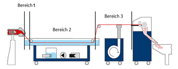
Figure 1: Exemplary strand cooling with additional strand extraction and granulation

In order to determine the temperature distribution over the strand length and the strand cross-section, it is discretized as follows:

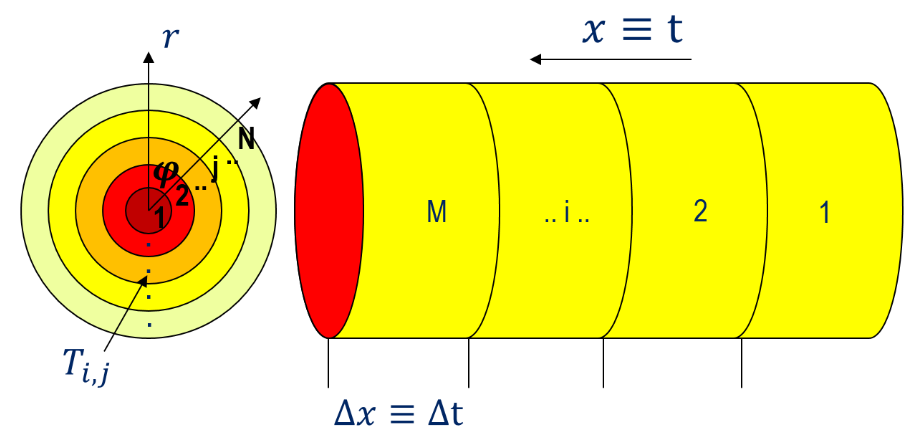
Figure 2: Discretization strand

In the length direction, the strand is divided into M segments with the running index i. Since the time is relevant for the unsteady heat conduction, it is described over the cooling length L and the line speed v.

The index i stands for any position x, at which the strand has already been in contact with the water for a specific time t. The length of the individual subintervals in the length direction can be determined with:

$$\Delta x = \frac{L}{M} \tag{1}$$

Further, the cross section in radial direction is divides into N segments with the index j. The subintervals with the radius of the strand R results to:

$$\Delta r = \frac{R}{N} \tag{2}$$

Therefore, the relevant temperatures have two indices ($T_{i,j}$) and are located in the middle of the defined intervals, see Figure 2.

To determine the time-related temperature fields within a solid, the Fourier differential equation is considered (here in cylinder coordinates) [VDI06]:

$$\rho c_p \frac{\partial T}{\partial t} = -\lambda \left[\frac{\partial^2 T}{\partial r^2} + \frac{1}{r} \frac{\partial T}{\partial r} + \frac{1}{r^2} \frac{\partial T}{\partial \varphi^2} + \frac{\partial^2 T}{\partial z^2}\right] \pm \dot{q}_s \tag{3}$$

For the current problem (viz. no external heat source, no angular temperature gradient), the differential equation is simplified as follows:

$$\frac{\partial T}{\partial t} = \frac{\lambda}{\rho \cdot c_p} \cdot \left[\frac{\partial^2 T}{\partial r^2} + \frac{1}{r} \frac{\partial T}{\partial r}\right] \tag{4}$$

The finite difference method provides an approximate solution, whereby the introduced error can be minimized by increasing the degree of discretization. However, this also increases the calculation effort. To approximate the partial derivatives, a Taylor series development is performed.

A Taylor series expansion is carried out to approximate the partial derivatives: The development of the temperature for a small time step results in [BK97]:

$$T_{t+\Delta t,r} = T_{t,r} + \frac{\partial T}{\partial t} \Delta t + \cdots \tag{5}$$

The Taylor series development is broken off after the first member, resulting in

$$\frac{\partial T}{\partial t} = \frac{T_{t+\Delta t,r} - T_{t,r}}{\Delta t} \tag{6}$$

The first of the three partial derivatives is approximated with

$$\frac{\partial T}{\partial t} = \frac{T_{t+\Delta t,r} - T_{t,r}}{\Delta t} = \frac{T_{i+1,j} - T_{i,j}}{\Delta t} \tag{7}$$

A Taylor series development of the temperature in the radial direction with truncation after the second element results in the following [BK97]:

$$T_{i,j+1} = T_{i,j} + \frac{\partial T}{\partial r} \Delta r + \frac{1}{2} \frac{\partial^2 T}{\partial r^2} \Delta r^2 + \cdots \tag{8}$$

$$T_{i,j-1} = T_{i,j} - \frac{\partial T}{\partial r} \Delta r + \frac{1}{2} \frac{\partial^2 T}{\partial r^2} \Delta r^2 + \cdots \tag{9}$$

These two equations are added together:

$$\frac{\partial^2 T}{\partial r^2} = \frac{T_{i,j+1} - 2T_{i,j} + T_{i,j-1}}{\Delta r^2} \tag{10}$$

Substituting equation 10 into equation 8 or equation 9 yields:

$$\frac{\partial T}{\partial r} = \frac{T_{i,j+1} - T_{i,j-1}}{2 \cdot \Delta r} \tag{11}$$

This determines all partial derivatives approximately. Inserting them into equation 4 gives the following result:

$$\frac{T_{i+1,j} - T_{i,j}}{\Delta t} = a \left[\frac{T_{i,j+1} - 2T_{i,j} + T_{i,j-1}}{\Delta r^2} + \frac{1}{r} \frac{T_{i,j+1} - T_{i,j-1}}{2 \cdot \Delta r}\right] \tag{12}$$

After a few simplifications, the following expression results:

$$T_{i+1,j} = T_{i,j} + \frac{\Delta t \cdot a}{R^2} \left[(T_{i,j+1} - 2T_{i,j} + T_{i,j-1}) \cdot N^2 + \frac{N}{j} \cdot \frac{T_{i,j+1} - T_{i,j-1}}{2}\right] \tag{13}$$

In addition, the time difference Δt can be described by the ratio of the length to the pull-off speed:

$$T_{i+1,j} = T_{i,j} + \frac{\Delta x \cdot a}{v_{ab} \cdot R^2} \left[(T_{i,j+1} - 2T_{i,j} + T_{i,j-1}) \cdot N^2 + \frac{N^2 T_{i,j+1} - T_{i,j-1}}{j \cdot 2}\right] \tag{14}$$

$$T_{i+1,j} = T_{i,j} + \frac{\Delta x \cdot a \cdot N^2}{v_{ab} \cdot R^2} \left[(T_{i,j+1} - 2T_{i,j} + T_{i,j-1}) + \frac{1}{j} \frac{T_{i,j+1} - T_{i,j-1}}{2}\right] \tag{14.1}$$

For each shell j, the material-specific properties are determined in each time step i depending on the temperature.

It can be seen that the temperature can be determined on the basis of three temperatures that are located in the preceding length segment i. If the temperature is to be determined in the last radial segment at j=N, there is no preceding temperature with the index j+1; similarly, there is no preceding temperature with j-1 in the middle of the line. Accordingly, boundary conditions must be defined for these limiting cases in order to calculate auxiliary temperatures.

It is assumed, that the initial strand temperature is constantly distributed over the cross section and corresponds to the temperature at the screw tip.

$$T_{0,j} = T_M \text{ for all j} \tag{15}$$

For all radial segments with index j=1, it is assumed that the two predecessor temperatures $T_{i,j}$ und $T_{i,j-1}$ are the same. The Taylor series development is broken off after the first member, resulting in equation 6:

$$T_{i+1,1} = T_{i,1} + \frac{\Delta x \cdot a}{v_{ab} \cdot R^2} \cdot (T_{i,2} - T_{i,1}) \cdot \frac{3}{2} \cdot N^2 \tag{16}$$

In the last radial segment j=N is no previous temperature with index j+1. Therefore, an auxiliary temperature is needed, which is linked to the water temperature. For this purpose, an auxiliary layer is defined, which is a step size (Δr) behind the last segment and represents the index j + 1.

The calculated temperatures are always at the core of the segments, see figure 2. This means für j=N, that the last segment is not the surface temperature. The surface is displaced by the length Δr/2.

To determine the temperature in the auxiliary layer, a boundary condition of the third kind (or Newton boundary condition) is considered, which is used for the convective heat transfer. The respective auxiliary temperature can be determined graphically, see figure 3. A Taylor series development of the temperature in the radial direction with truncation after the second element results in the following [BK97], [VDI06].

$$T_{i,Hilfs.} = T_{i,N} + \frac{\Delta r}{\frac{\lambda}{\alpha} + \frac{\Delta r}{2}} \cdot (T_U - T_{i,N}) \tag{17}$$

The distance is calculated from the equilibrium between the heat flow emitted to the environment and the heat flow supplied by the strand via heat conduction, compare [BK97]. For the calculation of the heat transfer coefficient and the therefor required Nusselt number, the case of a moving cylinder in a resting fluid with the assumption Pr = 10 is used [VDI06].

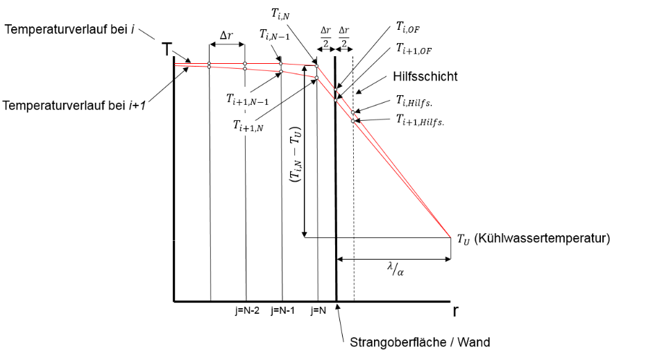
Figure 3: Exemplary temperature curves at I and i+1

Based on the Binder-Schmidt method (see [BK97]), the following boundary is defined for the factor (Fourier number) from equation 18:

$$\frac{\Delta t \cdot a}{\Delta r^2} \leq \frac{1}{2} \tag{18}$$

The following minimum value is specified for the axial number of segments:

$$N_{min} = \frac{\alpha \cdot R}{2\lambda} \tag{19}$$

$$M_{min} = N^2 \cdot 2 \cdot \frac{\lambda}{\rho \cdot c_p} \cdot \frac{L}{v_{ab} \cdot R^2} \tag{20}$$

After the calculation of the cooling length, SIGMA displays different temperatures. These temperatures are calculated as follows:

Core temperature:

$$T_{i,Mitte} = T_{i,1} \tag{21}$$

Surface temperature:

$$T_{i,OF} = \frac{(T_{i,N} + T_{i,Hilfs.})}{2} \tag{22}$$

Mean temperature:

$$T_{i,Mittel} = \frac{2}{N^2 + N} \cdot \sum_{j=1}^N j \cdot T_{i,j} \tag{23}$$

[BK97] Bosnjakovic, F.; Knoche, K. F.: „Technische Thermodynamik Teil II„; Dr. Dietrich Steinkopff Verlag, GmbH & Co. KG; Darmstadt; 1997

[FP08] Ferziger, J. H.; Peric, M.: „Numerische Strömungsmechanik“; Springer-Verlag Berlin Heidelberg; 2008

[Mar11] Martin, H.: „Numerische Strömungssimulation in der Hydrodynamik„; Springer-Verlag Berlin Heidelberg; 2011

[VDI06] Verein Deutscher Ingenieure: „VDI – Wärmeatlas“; Springer-Verlag Berlin Heidelberg; 2006